
Developing an error-correcting complementary modeling approach for surface water quality
Experiment name:
Developing an error-correcting complementary modeling approach for surface water quality
Scientific question:
Can we train data-driven algorithms to accurately detect systematic errors produced by process-based models?
Experiment idea:
This is a proof-of-concept for the development of hybrid modeling approaches in surface water quality modeling. The hybrid modeling approach integrates process-based hydrodynamic models with data-driven algorithms. The data-driven algorithm aims to capture and predict systematic errors in the process-based model predictions. This experiment evaluates the performance gains from this hybrid scheme in terms of mean and maximum errors.


![]()
Ilias PECHLIVANIDIS
[email protected]

Andrea VIRDIS
[email protected]

Blake SCHAEFFER
[email protected]
Background information
This is a proof-of-concept for the development of error-correcting complementary modeling approaches in surface water quality modeling. Although such hybrid modeling approaches have been applied successfully to problems related to surface water hydrology and groundwater modeling, there has been limited attention to their use for surface water quality problems. This experiment fills this gap by examining the potential of error-correcting data-driven models in the context of surface water quality.
The complementary modeling approach employed in this experiment integrates calibrated, process-based hydrodynamic models with data-driven algorithms to partially capture and predict systematic errors in the process-based model predictions. This experiment evaluates the performance gains from the inclusion of the error-correcting framework in terms of mean and maximum errors.
The error-correcting complementary models employed in this study integrate the calibrated process-based hydrodynamic models with (a) a random forest (RF) model and (b) a Gaussian Process Regression (GPR) algorithm to partially capture and predict systematic errors in the model predictions.
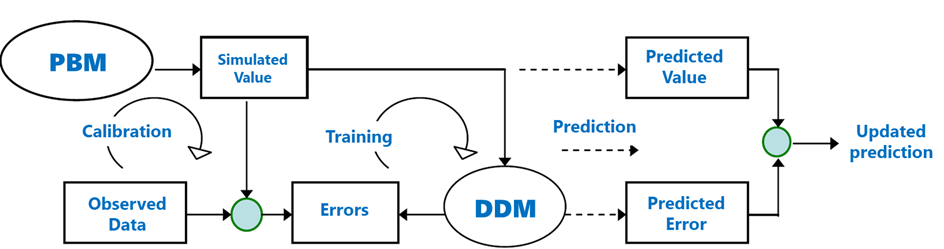
Schematic overview of the error-correcting framework.
A calibrated hydrodynamic model was used to simulate the relevant water quality attributes over a large period and the corresponding predicted errors are collected to formulate the target value. In this experiment, surface water temperature was the water quality attribute of interest.
Predicted errors were calculated from the deviation of predictions from the observed surface water temperatures. Surface water temperatures are estimated from satellite data using the MIP algorithm and Landsat-8 retrievals covering the period 2015-2019.
Data series comprising meteorological and hydrological variables are collected to formulate the input features of the data-driven models that will be developed. Meteorological variables contained total solar radiation, and air temperature, while hydrological variables included total inflows from the upstream catchments and water temperature.
The alternate models were trained using data from the period 2015-2018 and tested with the year 2019. Ultimately, a residual analysis is performed to evaluate the reduction of error in terms of their mean and maximum values.
Leader
EMVIS
Short Description
This task collects all the available data (EO, in situ, simulated) and formulates a data set that will be utilized for the model training and testing.
Outcome
A Matlab-based script is employed to formulate all data to produce the predictors and target values of the two different machine learning approaches.
This script initially reads all the relevant data from an HDF5 file that is available here: https://zenodo.org/record/7900605
An integral step of the prediction strategy involves the application of a lag and a sliding window method. The width of the moving window was arbitrarily selected equal to two days. To provide an example of how data are formulated in the prediction strategy, for the day-ahead prediction with a ten-day sliding window, (a) a one-day lag was applied to the target, and (b) the predictor matrix contained statistical indices of the hydrometeorological inputs of the last two days. These statistical indices were: (a) the total inflows entering the reservoir from the upstream catchment areas, (b) the mean temperature of the inflows entering the reservoir, (c) mean, maximum and minimum air temperature, and (d) cumulative solar radiation.
Leader
EMVIS
Short Description
Task 2 initially normalizes data using Z-score. Then, it splits the data into two partitions, the training, and the testing partitions.
Outcome
Initially, to account for the different scales between predictors (e.g., total precipitation values and total inflow from upstream catchment areas), the predictor set was normalized using Z-score. Z-scores measure the distance of a data point from the mean in terms of the standard deviation. The standardized data set has zero mean and standard deviation equal to one but retains the shape properties of the original data set (same skewness and kurtosis).
Following normalization, data were split into two partitions to safeguard against overfitting. These splits were performed as follows: (a) years 2015-2018 were used for training and, (b) year 2019 was used for testing.
The script is available here: https://github.com/EMVIS/ML-Forecasting
Leader
EMVIS
Short Description
This task optimizes the hyperparameters of an RF algorithm using a Bayesian optimization algorithm.
Outcome
A Matlab-based script was created to find the hyperparameters of the RF algorithm that minimize out-of-bag errors.
Model development was performed using surrogate splits and an interaction-curvature test for predictor selection, through the Treebagger function of Matlab. Hyperparameter optimization was performed through a Bayesian optimization algorithm (bayesopt function of Matlab). Four parameters were considered adjustable: the minimum leaf size (minLS), the number of variables to sample (nVars), the number of splits (nSplit), and the number of regression trees (nTree). When growing decision trees to create their ensemble, optimization targets for their simplicity and predictive power. Deep trees with many leaves are usually highly accurate on the training data. However, these trees are not guaranteed to show comparable accuracy for out-of-sample predictions. A leafy tree tends to overtrain (or overfit), and its out-of-sample accuracy is often far less than its training accuracy. In contrast, a shallow tree does not attain high training accuracy. But a shallow tree can be more robust — its training accuracy could be close to that of a representative test set. Also, a shallow tree is easy to interpret. In this regard, the adjustable parameters were constrained to provide shallow trees.
The script is available here: https://github.com/EMVIS/ML-Forecasting
Leader
EMVIS
Short Description
This task optimizes the hyperparameters of a GPR algorithm using a Bayesian optimization algorithm and five-fold cross validation.
Outcome
The GPR was trained using the fitrgp built-in function of Matlab.
Training a GPR model consists of specifying the most appropriate (a) formulation of the kernel function, (b) basis function, (c) the noise variance, and (d) hyperparameters that produce the best fit to the observed data.
Different kernel covariance functions were tested during GPR model training, all, however, considering the diverse length scale for each predictor (non-isotropic kernels); a different length scale allows for an estimation of relative predictor importance. The candidate kernel covariance functions were: (a) squared Exponential Kernel, (b) exponential Kernel, (c) rational quadratic Kernel, and (d) Matern 5/2 and 3/2 kernels.
Three basis functions were also considered: (a) constant, (b) linear, and (c) pure quadratic.
Ultimately, to avoid overfitting due to the low number of data available, hyperparameters θ, (i.e., length scales and signal standard deviations) were constrained in such way so that they could offer coarser approximations and narrow prediction intervals.
Leader
EMVIS
Short Description
This task uses the testing partition and the RF model (a) to estimate prediction errors and (b) correct surface water temperature predictions for year 2019.
Outcome
A Matlab-based script employs the predict function to estimate the RF-based hybrid solution under unseen conditions (year 2019). The data-driven and mechanistic outputs are added together, and corrected surface water temperatures are estimated.
Leader
EMVIS
Short Description
This task uses the testing partition and the GPR model (a) to estimate prediction errors and (b) correct surface water temperature predictions for year 2019.
Outcome
A Matlab-based script employs the predict function to estimate the GPR-based hybrid solution under unseen conditions (year 2019). The data-driven and mechanistic outputs are added together, and corrected surface water temperatures are estimated.
Leader
EMVIS
Short Description
This task aggregates temporally the mean and maximum errors provided by the error-correcting complementary modeling approaches.
Outcome
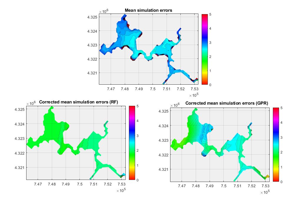
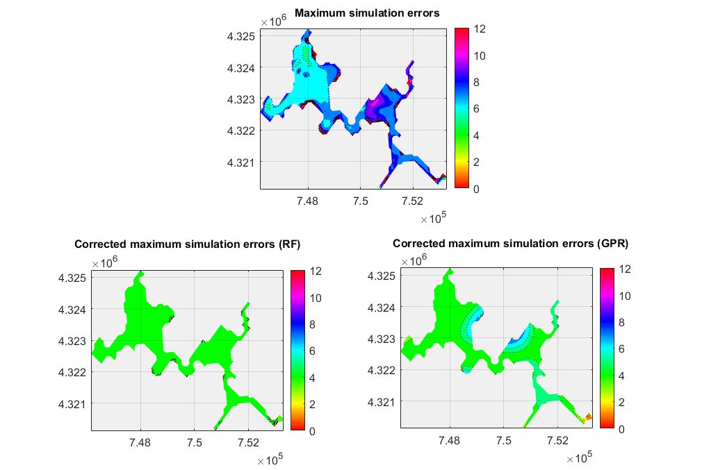
This task analyses the residuals from the two alternate hybrid solutions and compares them with the uncorrected outputs of the process-based model.
On average, the application of the error-correcting framework offered a sizeable error reduction regardless of the model approach. Uncorrected simulation errors were mostly between 2.2 oC and 3.2 oC; only a few near-shore areas demonstrated higher errors. The RF-based corrected errors varied from 1.2 oC to 1.8 oC, while their GPR-based counterparts were between 1.2 oC and 2.8 oC.
Maximum errors were reduced also reduced using the RF-based predictions. Uncorrected maximum errors were found between 6 oC and 11 oC. The RF-based solution reduced those errors in the range of 4 oC throughout the entire domain (minor exceptions exist in the riverine zones of the lake). The GPR algorithm achieved a similar reduction in most of the water body, however there were still areas in which maximum errors were as high as 7.1 oC.
In absolute terms, high errors were still produced even after the application of the error-correcting framework. This indicates that the variability of errors cannot be completely captured by the ML models.
This experiment demonstrated the potential of hybrid ML and process-based models in the prediction of surface water temperature in lakes and reservoirs.
Although a properly constructed and calibrated model can provide useful information about the system behavior, uncertainties involved in model development and parameterization lead to prediction errors that might be captured by data-driven models.
The process-based model is associated with conceptual, parameter, and measurement uncertainty. The calibrated hydrodynamic model resolved most of the physical processes satisfyingly, yet it missed some of the localized behaviors derived from heterogeneities and other sources of model uncertainties introduced into the system. The data-driven models then focused on predicting the resulting errors, which are assumed to reflect the unaccounted system behavior.
The resulting coupled models provided improved predictions. Compared to the purely process-based solution, hybrid solutions achieved three-fold lower mean absolute errors. This sizeable reduction was observed for both RF and GPR models tested herein. Regarding maximum absolute errors, the RF algorithm outperformed the GPR-based solution and managed to reduce maximum by nearly 2.5 times. The GPR model captured maximum errors for most of the lake, but in some areas, it failed to detect them accurately.
The error-correcting approach examined herein is not conditioned to any specific source of uncertainties. Thus, this approach is potentially gainful compared to other model updating techniques, especially if there are multiple sources of uncertainty that are hardly identifiable.
However, the effectiveness of the approach relies heavily on the prediction error patterns of the process-based model. This explains why the data-driven models performed differently in different areas of the case study considered. Models in areas with rare and high prediction errors underpredicted this type of error.
Leave a Reply
You must be logged in to post a comment.