
Quantile-based modeling of phytoplankton dynamics using Random Forests
Experiment name:
Quantile-based modeling of phytoplankton dynamics using Random Forests
Scientific question:
Can we improve the predictability of such events that occur at the limit of probability? If we can, how reliable is the prediction for a new instance?
Experiment idea:
This experiment tests how to implement Bayesian optimization to tune the hyperparameters of random forests using quantile errors. Tuning a model using quantile error, rather than mean squared error, is appropriate to use the model to predict conditional quantiles rather than conditional means.


![]()
Ilias PECHLIVANIDIS
[email protected]

Andrea VIRDIS
[email protected]

Blake SCHAEFFER
[email protected]
Background information
The frequency, magnitude, and duration of algae-related events in surface waters is increasing globally (Huisman et al., 2018), but still such events are rare and, in many cases, abrupt. Thus, water managers are limited in their ability to determine if, when, and where these events may be occurring.
A major scientific question arises from the frequency-of-occurrence of algae-related events. Can we improve the predictability of such events that occur at the limit of probability? If we can, how reliable is the prediction for a new instance?
To illustrate how these questions translate in decision-making, let us consider an example with the prediction of chlorophyll-a in a water reservoir. A typical regression problem would estimate the conditional mean of chlorophyll-a levels. Nonetheless, this estimate would provide limited insight on the fluctuations of chlorophyll-a levels around the predicted conditional mean. However, in many practical decision-making processes, it would be of interest to find a concentration level that is – with high probability – not surpassed. For such questions, quantile regression becomes relevant, as it goes beyond conditional mean predictions and gives information about the spread of the predictions.
Following the above conversation, this work aims to address the problem of predicting a quantile of the distribution of chlorophyll-a concentrations. Herein, we propose to adjust the model to the use of quantile loss as the objective function at the requested (by the end user) quantile levels.
This experiment develops quantile regression forests (QRFs) following the concept introduced by Meisenhausen (2006). QRFs are based on Breiman’s (2001) random forests. Random forests are regression algorithms that average an ensemble of decision trees. The ensemble is created by bagging regression trees using an additional randomization process. With this additional randomization, the splitting in the nodes of the regression tree is conducted by randomly selecting a fixed number of predictor variables. While regression forests can approximate the conditional mean of the dependent variable, quantile regression forests approximate its conditional quantiles. Diverging from other quantile regression algorithms, quantile regression forests are not based on the minimization of the quantile score. While random forests estimate the conditional mean by averaging the outcomes of the individual decision trees, quantile regression forests average the indicator functions of the event that the outcome of the decision tree in the test set is lower than a specified probability level. In other words, QRFs are developed exactly as RFs, but they convey different outputs.
In this experiment, two alternate families of QRFs were developed: (a) QRF01, which was optimized for mean values of chlorophyll-a (as in the previous section), and (b) a quantile-based QRF, QRF02, whose objective function was to capture the 90% quantile of chlorophyll-a.
The two families of QRFs were tested and evaluated in all case studies (i.e., Mulargia reservoir, Lake Harsha, and Lake Hume) considering (a) the difference between the cumulative distribution functions of the QRFs and the empirical CDF of the observations, (b) the reliability of the predictions, and (c) the sharpness of the predictions for a 90% nominal probability level during the hindcast period of 2015-2019.
Leader
EMVIS
Short Description
This task collects the available hydrometeorological (predictors) and phytoplankton-related data (target values) for the training of the ensemble learning algorithm at each case study.
Outcome
Hydrological data comprise nutrient fluxes from the upstream catchments. Hydrological data for the three case studies are available through the following link: https://www.primewater.eu/datasets/?_data_type=simulated-hydrology
Meteorological data comprise air temperature at 2 m above surface, solar radiation, total precipitation, and wind speed at 10 meters above surface. Near surface meteorological variables are derived from a bias-corrected reanalysis data set, which can be accessed through the Copernicus Climate Data Store at: https://cds.climate.copernicus.eu/cdsapp#!/dataset/derived-near-surface-meteorological-variables.
Satellite-derived concentrations of chlorophyll-a can be accessed through: (a) https://zenodo.org/record/4582339 for Mulargia, (b) https://zenodo.org/record/4581108t for William H Harsha Lake, and (c) https://zenodo.org/record/4581196 for Lake Hume. All data cover a five-year-long period, i.e., 2015-2019, and refer to Landsat-8 and Sentinel-2 retrievals.
Leader
EMVIS
Short Description
In this task, gridded data for (a) meteorological variables and (b) remotely sensed chlorophyll-a concentrations are formulated as time-series data corresponding to specific areas of interest (AOIs) within the water bodies.
Outcome
Remotely sensed chlorophyll-a concentrations were re-formatted as time series data by averaging chlorophyll-a concentrations within a radius of 200 m around specific areas of interest (AOIs).
For Mulargia reservoir, the AOI is located at (39.6072,9.2547) and corresponds to the water abstraction area of the reservoir.
For William H Harsha Lake two AOIs were specified. They were located at: (39.0367, -84.1381), and (39.020, -84.1311). The two AOIs specified herein represent the two diverse parts of the lake in the east and in the west.
Likewise, four AOIs were selected for Lake Hume. These are located (a) at Heywoods (-36.0711,147.0644), (b) close to the dam wall (-36.1076, 147.034), (c) at the northern part of Hume (-36.0346, 147.1100), and (d) near the Mitta-Mitta arm (-36.1841, 147.0666).
Near surface meteorological variables were estimated at the center of each AOI using the gridded data collected at Task 1 and a nearest neighbor approach through the interp2 command of Matlab®.
Matlab-based scripts for the formatting of input data as time series are available here: https://github.com/EMVIS/ML-Forecasting
The output data formatted in time series are available here: https://zenodo.org/record/7853095
Leader
EMVIS
Short Description
First, this task handles missingness and noise in the target values (i.e., chlorophyll-a). Then, it prepares the training data sets applying a lag and a sliding window strategy for the predictors and the target values. Finally, it normalizes predictors and target values using z-score.
Outcome
Due to their sparser temporal resolution and the quality-related challenges (e.g., aerosol or cloud contamination) they are facing, satellite-derived time-series contained missing and noisy data. We adopted a two-step approach to handle missingness and noise in those time series. First, we applied linear interpolation scheme; gaps larger than three days were not interpolated and left as missing values, as described in Metz et al. (2017). Then, we applied the Savitzky-Golay filter to smooth noisy inputs.
An integral step of the prediction strategy involved the application of a lag and a sliding window method. The width of the moving window is estimated based on a grid-based search method, where different moving windows are concerned, and cross-validation errors are estimated.
To provide an example of how data are formulated in the prediction strategy, for the day-ahead prediction with a ten-day sliding window, (a) a one-day lag was applied to the target values (the time series of chlorophyll-a concentrations), and (b) the predictor matrix contained statistical indices of the hydrometeorological inputs of the last ten days (i.e., the width of the moving window). These statistical indices were: (a) the cumulative mass fluxes of total nitrogen and total phosphorus entering the reservoir from the upstream catchment areas (please note that for AOIs with more than one upstream catchments, these mass fluxes are treated separately), (b) the percentage (%) of time during which wind speed exceeds 3.0 m/s – Binding et al. 2018 and Zhang et al. 2021 indicate that a wind-speed threshold of 3.0 m/s is relevant for algae dynamics in lakes and reservoirs, (c) mean air temperature, (d) cumulative solar radiation, and (e) total daily precipitation.
To account for the different scales between predictors (e.g., total precipitation values and total inflow from upstream catchment areas), the predictor set was normalized using Z-score. Z-scores measure the distance of a data point from the mean in terms of the standard deviation. The standardized data set has zero mean and standard deviation equal to one but retains the shape properties of the original data set (same skewness and kurtosis).
Following normalization, data were split into five partitions to allow for a 5-fold validation during training and safeguard against overfitting. These splits were realized with the cvpartition MATLAB function to obtain a quasi-random draw.
Matlab-based scripts for data pre-processing are available here: https://github.com/EMVIS/ML-Forecasting
Leader
EMVIS
Short Description
This task searches for a subset of the features in the full model with comparative predictive power through a wrapper method.
Outcome
A Matlab-based script was created to employ a wrapper method for sequential feature selection. Backward direction was used for the sequential search of features assessing the relative change in the cross-validation errors. A feature was removed from the predictor list when its removal induced a change in the cross-validation errors lower than 1% (relative tolerance).
Then, for each case study and each AOI, a subset of the hydrometeorological variables is selected for the development of the corresponding models.
Leader
EMVIS
Short Description
This task optimizes the hyperparameters of the alternate QRF algorithms for each case study and AOI.
Outcome
Two Matlab-based functions were created to find the hyperparameters of the alternate QRF algorithms.
The first function (developed for QRF01) is intended to develop a QRF that predicts conditional means. Thus, the training of QRF01 is based on the minimization of out-of-bag errors. The second function (developed for QRF02) is intended to develop a QRF that predicts conditional quantiles rather than conditional means. Therefore, the function trains the QRF using out-of-bag quantile errors. A 0.90 quantile probability was considered.
Model development in both cases was performed using surrogate splits and an interaction-curvature test for predictor selection, through the Treebagger function of Matlab. Hyperparameter optimization was performed through a Bayesian optimization algorithm (bayesopt function of Matlab). Four parameters were considered adjustable: the minimum leaf size (minLS), the number of variables to sample (nVars), the number of splits (nSplit), and the number of regression trees (nTree).
Leader
EMVIS
Short Description
This task evaluates the (a) the difference between the cumulative distribution function of the QRF and the empirical CDF of the observations, (b) the reliability of the predictions, and (c) the sharpness of the predictions for a 90% nominal probability level during the hindcast period of 2015-2019.
Outcome
Two Matlab-based functions assess the performance of the alternate QRFs.
The aim of probabilistic modelling is to maximize sharpness subject to reliability. Reliability refers to the statistical consistency between the probabilistic predictions and the observations. Reliability can be assessed by measuring the coverage of the prediction intervals, i.e., the percentage of observations included in these intervals.
Sharpness refers to the narrowness of the prediction intervals. The interpercentile range (IPR) will measure the width of the prediction intervals. Here we considered two different percentiles of nominal values (probability levels) 0.05, 0.95, for predicting the uncertainty distributions of the realized values of the series of the data set, namely the 90% central prediction intervals (PIs). The 90% central PIs provide information about their tails, which are important in terms of the risk of extremely high or extremely low outcomes. In this view, smaller values of this score indicate more useful probabilistic predictions.
Ultimately, for the overall performance of the cumulative distribution function (CDF) produced by each QRF, the continuous rank probability score (CRPS) will be evaluated. CRPS measures the difference between the CDFs of the predictions and the empirical cumulative distribution functions (ECDFs) of observations. It ranges from 0 to infinity with lower values representing a better score. It collapses to the mean absolute error for deterministic forecasts.
Leader
EMVIS
Short Description
This task compares the probabilistic predictions of the two QRFs in the different case studies.
Outcome
Mulargia
Quantile-based regression resulted in random forests fewer but shallower trees: QRF02 contained 96 decision trees with a minimum leaf size of 45.
Probably due to this fact, QRF02 captured the variability of chlorophyll-a slightly worse compared to QRF01, demonstrating a nearly three-fold CRPS value. QRF01 was also better in terms of the reliability of the predictions, while the evaluated IPR was smaller. It should be noted that the reliability score for both cases was high, greater than 95%, which is considered the target value. Conclusively, even if QRF02 was optimized to minimize 0.90 quantile errors, the predictive performance was marginally lower.
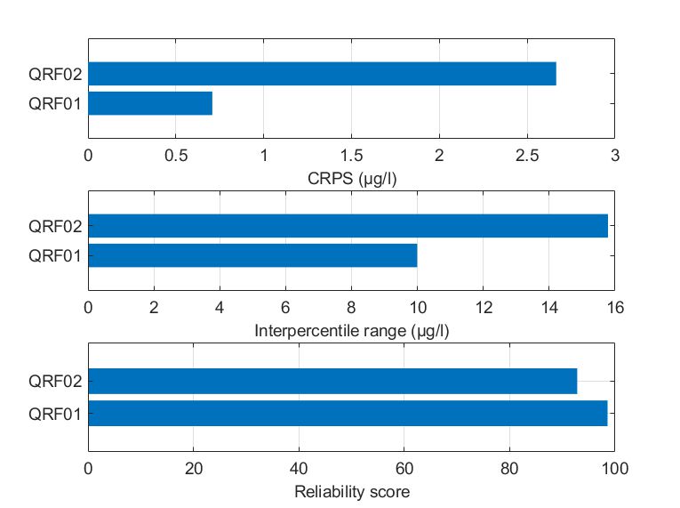
Figure Comparison of the two alternate quantile regression forests for the held-out data in Mulargia reservoir in terms of (a) CRPS values, (b) interpercentile range, and (c) reliability.
Harsha
As in the Mulargia case study, for both AOIs, quantile-based ensembles consisted of a few shallow trees. The mean leaf size was 45 for both AOIs.
For AOI1, both QRFs achieved similar reliability scores (higher than 95%), yet QRF02 demonstrated slightly lower IPR values. Nonetheless, the IPR values are considered unacceptably high for both formulations. In terms of the overall CDF performance, QRF02 performed marginally better with a slightly lower CPRS value compared to QRF01. Conclusively, both QRFs had high reliability scores but with similarly large IPR values.
For AOI2, QRF02 was marginally worse in terms of the achieved CRPS but demonstrated less reliable predictions for a 90% prediction interval. In both QRFs, the predictions did not capture adequately the variability of chlorophyll-a values (reliability scores were below 90%), while the IQR values were again high.
Conclusively, the sharpness of probabilistic predictions was slightly improved using quantile errors, however, there is no firm evidence supporting that this approach is clearly towards the right direction in terms of the prediction of higher quantiles.
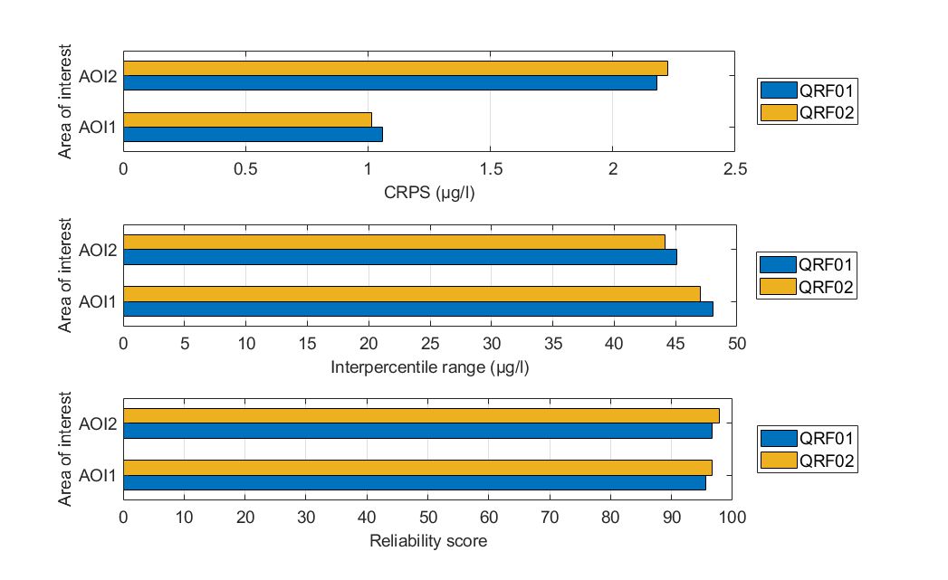
Figure. Comparison of the two alternate quantile regression forests for the held-out data in Lake Harsha in terms of (a) CRPS values, (b) interpercentile range, and (c) reliability.
Hume
The parameter fine-tuning of the quantile-based QRFs resulted in relatively similar formulations for all AOIs in Lake Hume. Through quantile regression, QRFs were based on relatively small ensembles (less than 400 decision trees were used) of shallow decision trees.
Regarding the overall performance of the QRFs in terms of their CDFs, QRF02 models were outperformed by QRF01 models. In terms of the sharpness of the predictions, QRF02 solutions were worse compared to QRF01 (wider prediction intervals). In terms of the reliability of the predictions, both formulations offered comparable results, which were higher than the desired level of 90%. Overall, training the QRF with quantile errors rather than conditional means did not induce any benefits in terms of the predictive abilities of the model.
To sum up, involving quantile errors in the development QRFs did not offer strong evidence supporting the predictions are more reliable and informative compared to QRFs developed to predict conditional means.
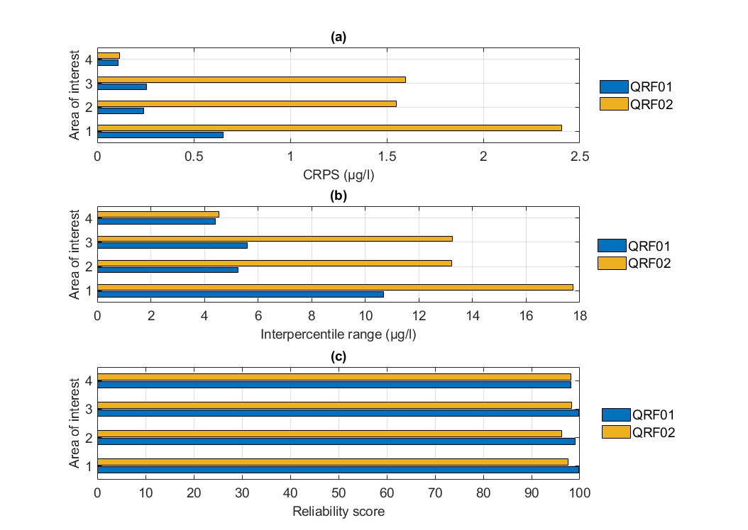
Figure. Comparison of the two alternate quantile regression forests for the held-out data in Lake Hume in terms of (a) CRPS values, (b) intepercentile range, and (c) reliability.
The effort to develop generalizable models could hamper the ability to predict accurately the magnitude of rare events of increased chlorophyll-a in freshwater reservoirs and lakes. Therefore, this experiment asked if the predictability of such events that occur at the limit of probability could be increased using quantile-based QRFs.
For this type of questions, the approach tested herein is a conceptually straightforward alternative to typical Bayesian approaches that are used for probabilistic predictions.
Two alternate QRFs were developed, a QRF optimized to predict conditional means, and a QRF optimized to predict conditional quantiles. The two QRFs were developed in all AOIs across the three cases studies, i.e., Mulargia reservoir, Lake Harsha, and Lake Hume. The QRFs were tested in terms of (a) the comparison of the predicted CDFs with the empirical CDFs of the observations, and (b) the reliability and sharpness of predictions for a nominal probability level of 90%.
From the training of the two alternate QRFs, it is evident that QRF trained with out-of-bag quantile errors required smaller ensembles of shallower decision trees compared to the QRFs trained with out-of-bag errors. In this case, this difference had negligible impact in the computational burden associated with the predictions, but in other applications the size of the ensemble of decision trees could be relevant.
When compared to each other, the two QRFs demonstrated (a) comparable reliability for a 90% nominal probability level, and (b) similar sharpness, which was estimated by the average width of the prediction intervals. It should be noted that the reliability of the predictions was in most cases at the desired levels (90%).
In terms of the produced CDFs, quantile-based QRFs offered minimal benefits for the tails of the ECDFs of the observations compared to the traditional regression-based QRFs in a few cases. The tails of the ECDFs are important in terms of the risk of extremely high outcomes, i.e., phytoplankton blooms. However, no general conclusions can be drawn from this experiment.
Overall, given the complexity of the processes simulated and the relatively imbalanced data available, predicting accurately high chlorophyll-a values cannot be solely addressed with changes in the objective function during parameter fine-tuning. The curse of dimensionality remains and, thus, larger data sets would be a solution in the right direction.
Leave a Reply
You must be logged in to post a comment.