
Assess the relevance of hydrometeorological variables in phytoplankton dynamics of surface waters using data-driven modeling
Experiment name:
Assess the relevance of hydrometeorological variables in phytoplankton dynamics of surface waters using data-driven modeling
Scientific question:
Can we use data-driven algorithms to gain insight into the drivers of phytoplankton dynamics in lake and reservoir ecosystems?
Experiment idea:
Data-driven models typically compromise interpretability for accuracy. While models in diverse domains might be evaluated solely in terms of predictive accuracy and speed, scientific models should be assessed by additional factors, such as a minimal number of parameters or its adherence to the mechanisms behind the processes. In our case, a model that does not abide by well documented mechanisms of phytoplankton dynamics, cannot be communicated clearly, except from computer to computer. As a result, its contribution to real-world decision-making would be insignificant. On the other hand, a model with an explanation for why it possesses the uncertainty it has is less likely to result in unpleasant surprises later. In this regard, this experiment asks whether the use of machine learning tools can help discover hidden trends in data and make meaningful predictions.
To this end, an ensemble learning algorithm is developed to assess the relevance of external forcings (i.e., hydrology and meteorology) in the prediction of phytoplankton dynamics in surface water reservoirs and lakes.
First, the experiment trains the ensemble learning algorithms for the prediction of chlorophyll-a values. Then, it utilizes variable importance metrics to assess the interrelation of hydrometeorological predictors and their relevance in the prediction of phytoplankton dynamics. Ultimately, model-agnostic tools (individual conditional expectation plots and Shapley values) are used to shed light upon the model’s internals aiming to decipher which hydrometeorological variables are critical for the prediction of phytoplankton dynamics in the water bodies.


![]()
Ilias PECHLIVANIDIS
[email protected]

Andrea VIRDIS
[email protected]

Blake SCHAEFFER
[email protected]
Background information
Data-driven models typically compromise interpretability for accuracy. They are hardly interpretable unless the data is of low dimension. In such cases, any window into the model’s internals can be beneficial.
Random forests (RFs) offer such windows, as they can uncover interaction effects among variables, mainly due to the recursive structure of trees, which enables them to consider dependencies hierarchically. A divergent behavior in two branches of a tree after a split indicates possible interactions between the predictor variables. This experiment exploits this feature of RFs to unveil variable interaction effects in predicting chlorophyll-a concentrations observed remotely from multi-spectral satellite imagery.
The RF algorithm assesses the relevance of external forcings (hydrological and meteorological) in predicting accurately chlorophyll-a concentrations in specific areas of interest through a permutation variable importance metric (VIM). A permutation VIM measures the mean decrease in accuracy in the out-of-bag sample by randomly permuting the predictor variable of interest. If a predictor is influential in prediction, then permuting its values should drop model accuracy and high VIM values should be anticipated. On the contrary, if a predictor is not influential, then permuting its values should have little to no effect on the model error and VIMs will be distributed around zero (Strobl et al., 2009). For a detailed discussion on permutation VIMs and RFs, the reader should refer to Nicodemus et al. (2010).
In addition to the VIM, a model-agnostic visualization tool, i.e., the partial dependence plots (PDPs), will also be employed to gain insight into the model’s internals. Partial dependence plots (PDPs) are a way to visualize how the target variable (output) depends on a set of input variables (features) of a machine learning model. They show how the predicted outcome changes as we vary one or two features while keeping all other features constant. PDPs can help us understand the relationship
between the target variable and the input variables, and identify which features are most important for making predictions. In the presence of substantial interaction effects however, the partial response relationship can be heterogeneous. Individual conditional expectation (ICE) plots refine the partial dependence plot and suggest where and to what extent heterogeneities might exist.
Lastly, the Shapley value of a predictor, in the context of machine learning prediction, will evaluate the contribution of the predictor to a prediction. For each prediction, the sum of the Shapley values for all predictors corresponds to the total deviation of the prediction from the average. Thus, the Shapley values of all predictors provide an inkling of their relevance in the prediction of extremes.
The experiment will be performed for a 5-year-long period (2015-2019) in Mulargia reservoir, William H Harsha Lake, and Lake Hume. The data-driven algorithms will be trained on simulated hydrological data (nutrient loadings), simulated meteorological data (time series data of wind speed, air temperature, precipitation, and solar radiation) and remotely sensed chlorophyll-a (from Landsat-8 and Sentinel-2).
Leader
EMVIS
Short Description
This task collects the available hydrometeorological (predictors) and phytoplankton-related data (target values) for the training of the ensemble learning algorithm at each case study.
Outcome
Hydrological data comprise nutrient fluxes from the upstream catchments. Hydrological data for the three case studies are available through the following link: https://www.primewater.eu/datasets/?_data_type=simulated-hydrology
Meteorological data comprise air temperature at 2 m above surface, solar radiation, total precipitation, and wind speed at 10 meters above surface. Near surface meteorological variables are derived from a bias-corrected reanalysis data set, which can be accessed through the Copernicus Climate Data Store at: https://cds.climate.copernicus.eu/cdsapp#!/dataset/derived-near-surface-meteorological-variables.
Satellite-derived concentrations of chlorophyll-a can be accessed through: (a) https://zenodo.org/record/4582339 for Mulargia, (b) https://zenodo.org/record/4581108 for William H Harsha Lake, and (c) https://zenodo.org/record/4581196 for Lake Hume. All data cover a five-year-long period, i.e., 2015-2019, and refer to Landsat-8 and Sentinel-2 retrievals.
Leader
EMVIS
Short Description
In this task, the gridded data for (a) meteorological variables and (b) remotely sensed chlorophyll-a concentrations are formulated as time-series data corresponding to specific areas of interest (AOIs) within the water bodies.
Outcome
Remotely sensed chlorophyll-a concentrations were re-formatted as time series data by averaging chlorophyll-a concentrations within a radius of 200 m around specific areas of interest (AOIs).
For Mulargia reservoir, the AOI is located at (39.6072,9.2547) and corresponds to the water abstraction area of the reservoir.
For William H Harsha Lake two AOIs were specified. They were located at: (39.0367, -84.1381), and (39.020, -84.1311). The two AOIs specified herein represent the two diverse parts of the lake in the east and in the west.
Likewise, four AOIs were selected for Lake Hume. These are located (a) at Heywoods (-36.0711,147.0644), (b) close to the dam wall (-36.1076, 147.034), (c) at the northern part of Hume (-36.0346, 147.1100), and (d) near the Mitta-Mitta arm (-36.1841, 147.0666).
Near surface meteorological variables were estimated at the center of each AOI using the gridded data collected at Task 1 and a nearest neighbor approach through the interp2 command of Matlab®.
Matlab-based scripts for the formatting of input data as time series are available here: https://github.com/EMVIS/ML-Forecasting
The output data formatted in time series are available here: https://zenodo.org/record/7780519#.ZFoFIRFBzIU
Leader
EMVIS
Short Description
First, this task handles missingness and noise in the target values (i.e., chlorophyll-a). Then, it prepares the training data sets applying a lag and a sliding window strategy for the predictors and the target values. Finally, it normalizes predictors and target values using z-score.
Outcome
Due to their sparser temporal resolution and the quality-related challenges (e.g., aerosol or cloud contamination) they are facing, satellite-derived time-series contained missing and noisy data. We adopted a two-step approach to handle missingness and noise in those time series. First, we applied linear interpolation scheme; gaps larger than three days were not interpolated and left as missing values, as described in Metz et al. (2017). Then, we applied the Savitzky-Golay filter to smooth noisy inputs.
An integral step of the prediction strategy involved the application of a lag and a sliding window method. The width of the moving window is estimated based on a grid-based search method, where different moving windows are concerned, and cross-validation errors are estimated.
To provide an example of how data are formulated in the prediction strategy, for the day-ahead prediction with a ten-day sliding window, (a) a one-day lag was applied to the target values (the time series of chlorophyll-a concentrations), and (b) the predictor matrix contained statistical indices of the hydrometeorological inputs of the last ten days (i.e., the width of the moving window). These statistical indices were: (a) the cumulative mass fluxes of total nitrogen and total phosphorus entering the reservoir from the upstream catchment areas (please note that for AOIs with more than one upstream catchments, these mass fluxes are treated separately), (b) the percentage (%) of time during which wind speed exceeds 3.0 m/s – Binding et al. 2018 and Zhang et al. 2021 indicate that a wind-speed threshold of 3.0 m/s is relevant for algae dynamics in lakes and reservoirs, (c) mean air temperature, (d) cumulative solar radiation, and (e) total daily precipitation.
To account for the different scales between predictors (e.g., total precipitation values and total inflow from upstream catchment areas), the predictor set was normalized using Z-score. Z-scores measure the distance of a data point from the mean in terms of the standard deviation. The standardized data set has zero mean and standard deviation equal to one but retains the shape properties of the original data set (same skewness and kurtosis).
Following normalization, data were split into five partitions to allow for a 5-fold validation during training and safeguard against overfitting. These splits were realized with the cvpartition MATLAB function to obtain a quasi-random draw.
Matlab-based scripts for data pre-processing are available here: https://github.com/EMVIS/ML-Forecasting
Leader
EMVIS
Short Description
This task searches for a subset of the features in the full model with comparative predictive power through a wrapper method.
Outcome
A Matlab-based script was created to employ a wrapper method for sequential feature selection. Backward direction was used for the sequential search of features assessing the relative change in the cross-validation errors. A feature was removed from the predictor list when its removal induced a change in the cross-validation errors lower than 1% (relative tolerance).
Then, for each case study and each AOI, a subset of the hydrometeorological variables is selected for the development of the corresponding models.
Leader
EMVIS
Short Description
This task optimizes the parameters of the RF algorithm as an ensemble regression learner for each case study and AOI.
Outcome
A Matlab-based script was created to find the hyperparameters of the RF algorithm that minimize the cross-validation errors of chlorophyll-a predictions.
Model development was performed using surrogate splits and an interaction-curvature test for predictor selection, through the Treebagger function of Matlab. Hyperparameter optimization was performed through a Bayesian optimization algorithm (bayesopt function of Matlab). Four parameters were considered adjustable: the minimum leaf size (minLS), the number of variables to sample (nVars), the number of splits (nSplit), and the number of regression trees (nTree).
When growing decision trees to create their ensemble, optimization targets for their simplicity and predictive power. Deep trees with many leaves are usually highly accurate on the training data. However, these trees are not guaranteed to show comparable accuracy for out-of-sample predictions. A leafy tree tends to overtrain (or overfit), and its out-of-sample accuracy is often far less than its training accuracy. In contrast, a shallow tree does not attain high training accuracy. But a shallow tree can be more robust — its training accuracy could be close to that of a representative test set. Also, a shallow tree is easy to interpret. In this regard, the adjustable parameters were constrained to provide shallow trees.
Leader
EMVIS
Short Description
This task estimates for each model the variable importance metrics by permutation.
Outcome
Following model development and for every model, the corresponding permutation VIMs are calculated. Permutation VIMs allow for the global interpretability assessment of the model.
Leader
EMVIS
Short Description
This task produces PDPs and ICE plots for the predictors with the highest VIM values.
Outcome
For each predictor and for the entire dataset, the PDPs and ICE plots are produced using the plotpartialdepence in Matlab.
Leader
EMVIS
Short Description
This task estimates Shapley values for all chlorophyll-a predictions provided by the data-driven solutions.
Outcome
A MATLAB-based script was prepared to estimate the Shapley values for chlorophyll-a predictions.
Leader
EMVIS
Short Description
This task interprets chlorophyll-a predictions using local and global interpretability approaches.
Outcome
Mulargia
The developed RF model captured the temporal variability of chlorophyll-a with reasonable accuracy. The model slightly underpredicted the peak chlorophyll-a values that were observed from 2018 and onwards. Nonetheless, cross-validation errors were acceptable.
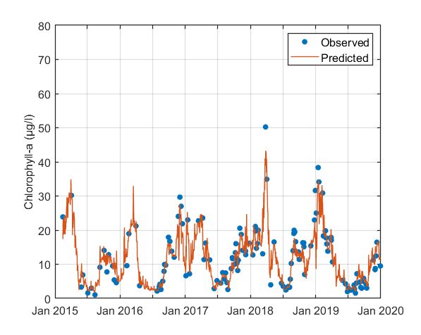
Figure. Observed versus cross-validation predictions of chlorophyll-a.
The sequential feature selection indicated that total precipitation and total nitrogen concentrations could be omitted from the feature list. The permutations VIMs estimated for the developed RF demonstrated that cumulative solar radiation and air temperature were the most influential parameters.
These findings were further corroborated by the estimated Shapley values. Shapley values implied that the contribution of wind speed and total phosphorus in phytoplankton dynamics is relatively low but cannot be ignored.
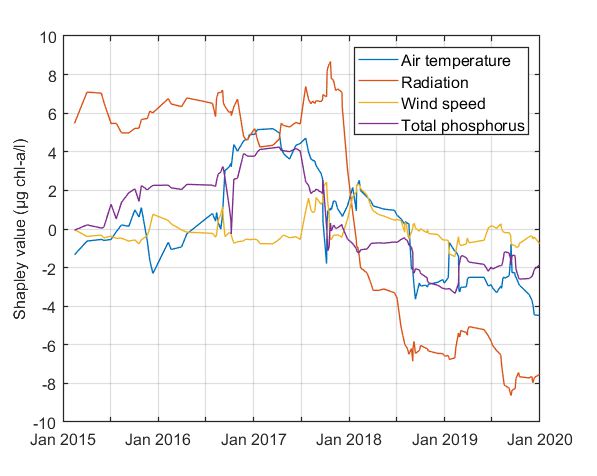
Figure. Shapley values for the predicted chlorophyll-a values.
Lastly, PDPs and ICE plots indicated that low air temperatures and moderate cumulative solar radiation values lead to increased chlorophyll-a concentrations at the top layers of the water column in the AOI. For the remaining features (wind speed and total phosphorus mass fluxes), there exist substantial heterogeneities. However, for the contribution of wind, the ICE plot unveils that for chlorophyll-a values exceeding 20 ug/l, vertical mixing due to increased wind speeds could impact chlorophyll-a concentrations positively.
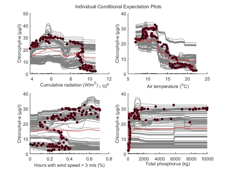
Figure. ICE plots for (a) cumulative solar radiation, (b) air temperature, (c) wind speed, and (d) total phosphorus mass fluxes. Red lines depict the partial dependence of each variable with chlorophyll-a.
Harsha
AOI1
The RF model described the observed chlorophyll-a values poorly. It suffered from under-fitting. Predicted chlorophyll-a values fluctuate between 10 ug/l to 40 ug/l, while observed values range from near-zero concentrations to nearly 80 ug/l. Limited data availability did not allow for the RF model to capture the few abnormal (low or high) values.
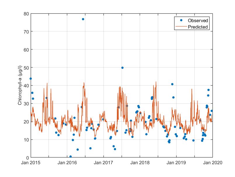
Figure. Observed versus cross-validation predictions of chlorophyll-a.
Sequential feature selection allowed for the removal of total nitrogen mass fluxes from the feature list. The permutations VIMs estimated for the developed RF demonstrated that cumulative solar radiation was the most influential parameter.
Limited data availability is reflected also in the interpretation of the predictions. Based on the computed Shapley values, summer chlorophyll-a outbreaks are attributed to radiation values. However, for the remaining periods of time, predictions are predicted through obscure patterns of the predictors.
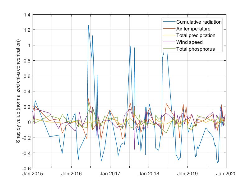
Figure. Shapley values for the predicted chlorophyll-a values.
This erratic behavior is further confirmed by the estimated ICE plots. Only radiation offered a meaningful relationship with chlorophyll-a concentrations. Increased chlorophyll-a concentrations were coupled with higher radiation values. This could also explain the tendency of the model to predict bloom events during summer months.
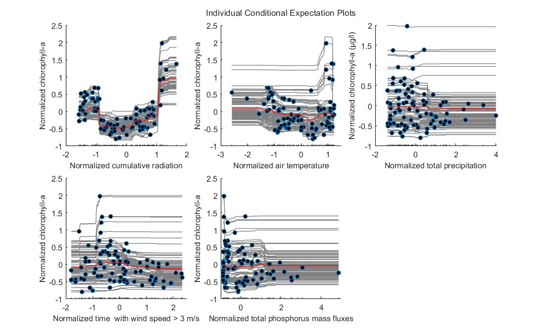
Figure. ICE plots for (a) cumulative radiation, (b) air temperature, (c) total precipitation, (d) wind speed, and (e) total phosphorus mass fluxes. Red lines depict the partial dependence of each variable with chlorophyll-a. Values in horizontal and vertical axes are normalized using z-scores.
AOI2
As in AOI1, the RF model did not predict the observed chlorophyll-a values adequately due to under-fitting. Again, predicted chlorophyll-a values fluctuate between 10 ug/l to 40 ug/l, while observed values range from near-zero concentrations to nearly 80 ug/l. Data availability was again a major issue, as it did not allow for the RF model to capture the few abnormal (low or high) values.
Sequential feature selection did not reduce the features of the model, as opposed to AOI 1. Permutations VIMs indicated that cumulative radiation is the most influential parameter. The remaining parameters are of similar importance for the model’s internal structure.
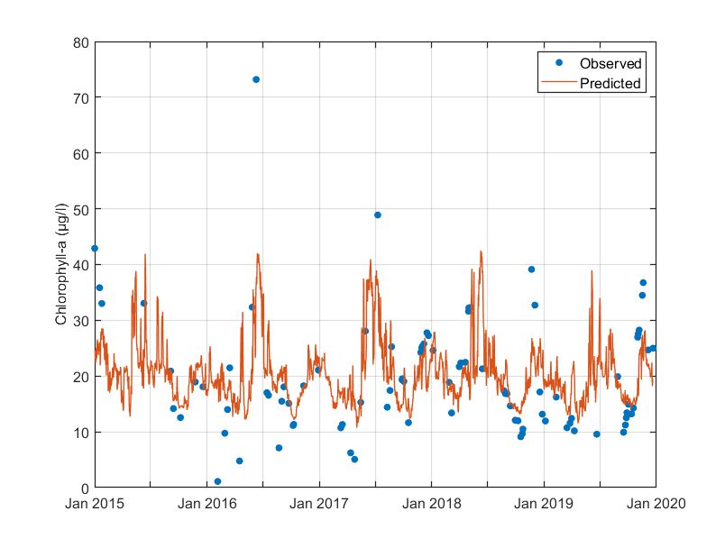
Figure. Observed versus cross-validation predictions of chlorophyll-a.
Due to the few data available, the model is hard to interpret, besides the summer peak values. Based on the computed Shapley values, summer chlorophyll-a outbreaks are attributed to increased radiation values. However, for the remaining periods of time, predictions are too complex to be interpreted.
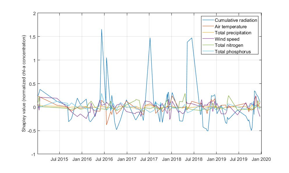
Figure. Shapley values for the predicted chlorophyll-a values.
This behavior is further confirmed by the estimated ICE plots and the PDPs. Again, it was only cumulative radiation that offered a meaningful relationship with chlorophyll-a concentrations.
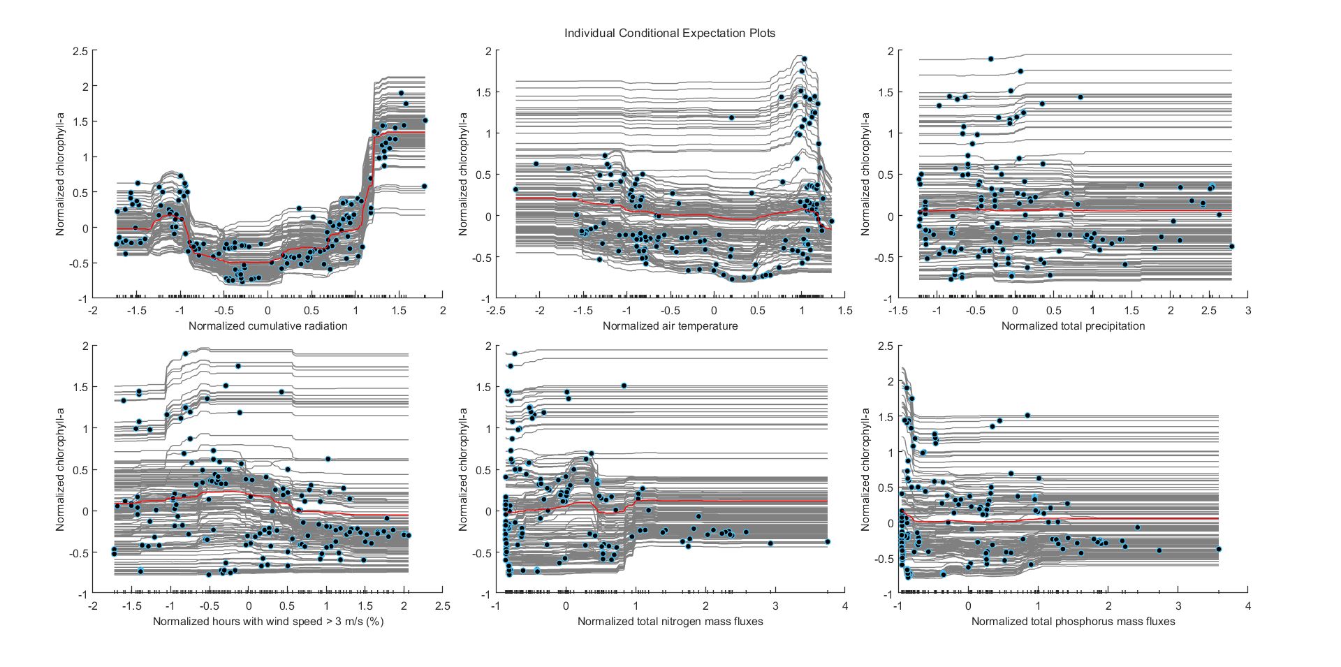
Figure. ICE plots for (a) cumulative radiation, (b) air temperature, (c) total precipitation, (d) wind speed, (e) total nitrogen mass fluxes, and (f) total phosphorus mass fluxes. Red lines depict the partial dependence of each variable with chlorophyll-a. Values in horizontal and vertical axes are normalized using z-scores.
Conclusively, for Lake Harsha modeling efforts are plagued by data availability (few than 100 data points are available) and suffer from underfitting issues. Based on the local and global interpretation of model predictions, cumulative radiation influences phytoplankton dynamics; increased radiation is expected to lead to higher chlorophyll-a concentrations. However, given the limited data available, the models were not able to capture all the underlying patterns and relationships in the data. Besides summer months, predictions are more complex and harder to understand.
Hume
AOI1
The developed model captured the temporal variability of chlorophyll-a with reasonable accuracy. Cross-validation errors were acceptable, capturing the timing of the 2016 bloom event.
Based on feature selection, air temperature and total phosphorus from catchment 2 were omitted from the feature list. Permutation VIMs suggest that nutrient mass fluxes (mostly total nitrogen) are the most influential parameters for chlorophyll-a predictions at AOI1.
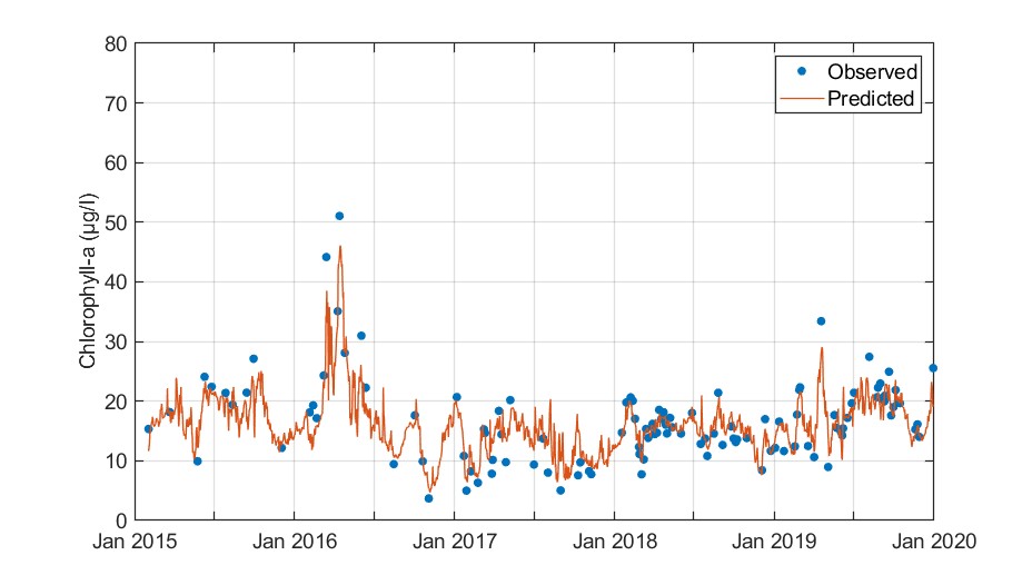
Figure. Observed versus cross-validation predictions of chlorophyll-a.
Shapley value confirmed the VIMs. Total nitrogen mass fluxes from the two upstream catchments are contributing mostly to chlorophyll-a predictions. This applies also for the 2016 bloom event. Total phosphorus is also relevant, while wind speed and total precipitation cannot be neglected. Nonetheless, Shapley values could not help us draw a more concrete conclusion on how these parameters impact chlorophyll-a predictions.
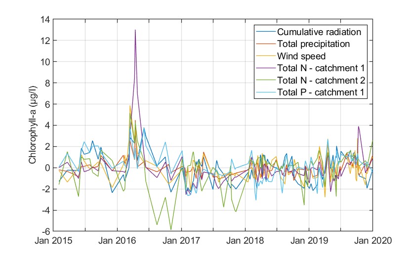
Figure. Shapley values for the predicted chlorophyll-a values.
ICE plots and PDPs unveiled sizable heterogeneities on the way that each parameter influences chlorophyll-a predictions for AOI1. These heterogeneities underscore that conclusions on the drivers of chlorophyll-a formation in AOI1 cannot be generalized through the RF model with certainty.
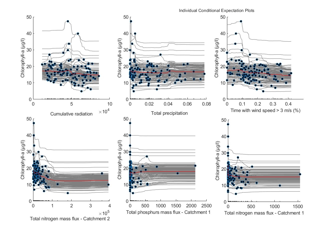
Figure. ICE plots for (a) cumulative radiation, (b) air temperature, (c) total precipitation, (d) wind speed, and (e) total phosphorus mass fluxes. Red lines depict the partial dependence of each variable with chlorophyll-a.
AOI2
The RF model described the temporal dynamics of chlorophyll-a formation adequately.
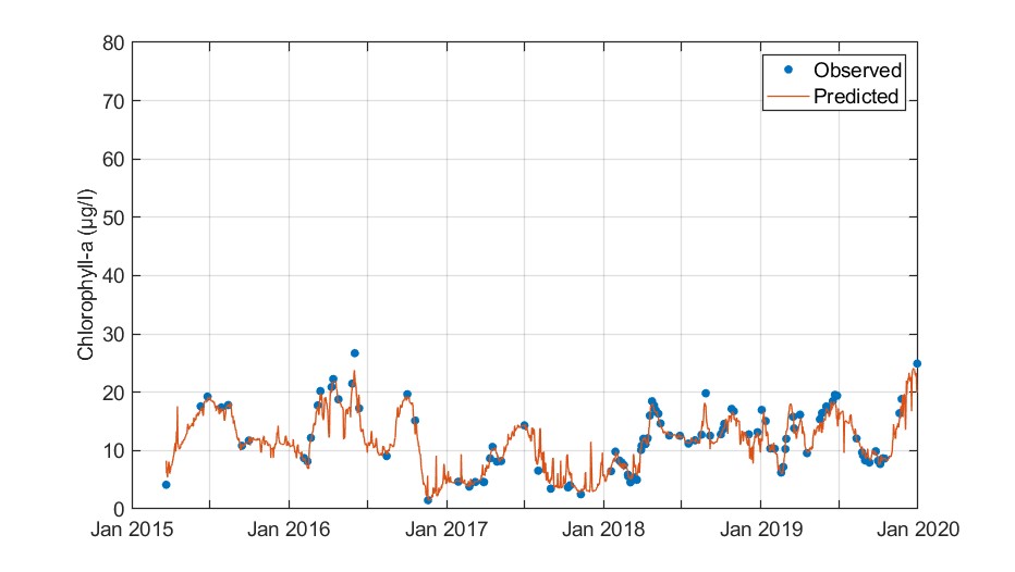
Figure. Observed versus cross-validation predictions of chlorophyll-a.
From the available features, only total phosphorus influxes from catchment 2 could be neglected without compromising predictive accuracy. Permutation VIMs indicate that all parameters are comparably significant for the model’s structure. Cumulative radiation and nutrient influxes were marginally more important.
Shapley values corroborate this remark. Cumulative radiation, total phosphorus, and total nitrogen mass fluxes appear to influence substantially chlorophyll-a predictions, both positively and negatively. However, Shapley values also highlight that a more general pattern for phytoplankton dynamics cannot be easily discovered. The same conclusions are drawn from the ICE plots and the PDPs of each variable.
Figure. Shapley values for the predicted chlorophyll-a values.
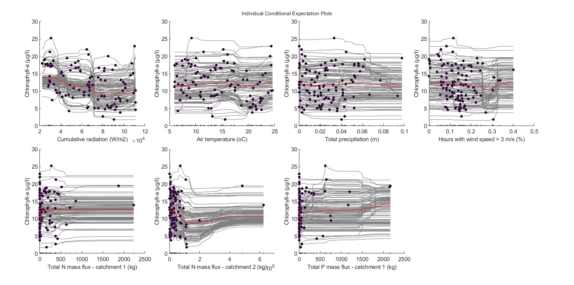
Figure. ICE plots for (a) cumulative radiation, (b) air temperature, (c) total precipitation, (d) wind speed, (e-f) total nitrogen mass fluxes, and (g) total phosphorus mass fluxes. Red lines depict the partial dependence of each variable with chlorophyll-a.
AOI3
The model developed for AOI3 provided low cross-validation errors.
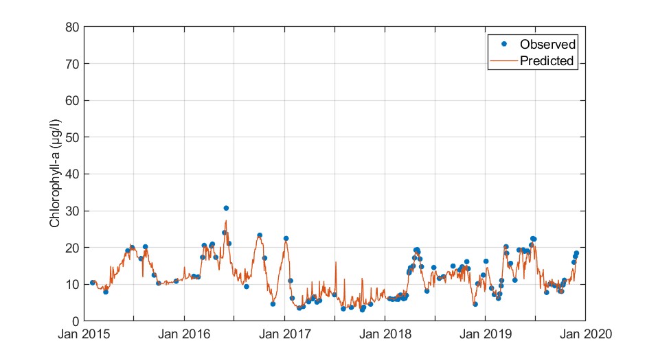
Figure. Observed versus cross-validation predictions of chlorophyll-a.
Permutation VIMs from the RF model indicate that radiation, and total nutrient influxes from catchment 1 are critical components of the model’s internal structure.
Shapley values confirm the relevance of these features. Cumulative radiation, total phosphorus fluxes, and total nitrogen fluxes from catchment 1 substantively impact chlorophyll-a variability, both positively and negatively. As in the previous AOIs for lake Hume, Shapley values also highlight that a clear pattern for phytoplankton dynamics in AOI3 cannot be easily revealed.
ICE plots and the PDPs implied that there is a tendency for chlorophyll-a to be coupled with increased total P fluxes, but they also revealed sizeable heterogeneities in the way that each parameter impacts chlorophyll-a predictions.
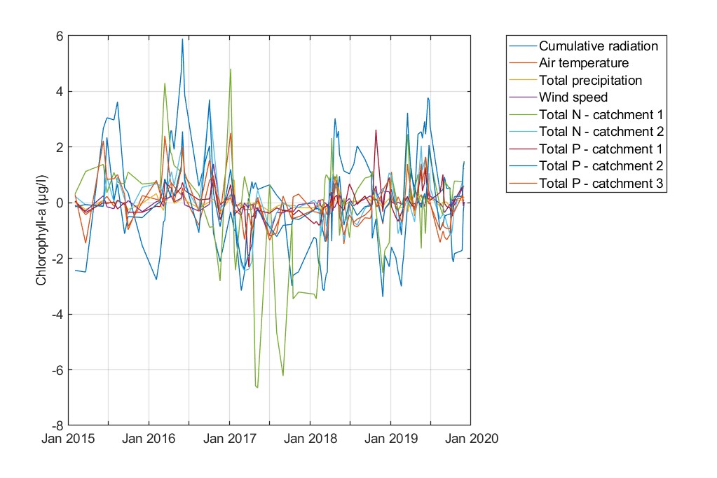
Figure. Shapley values for the predicted chlorophyll-a values.
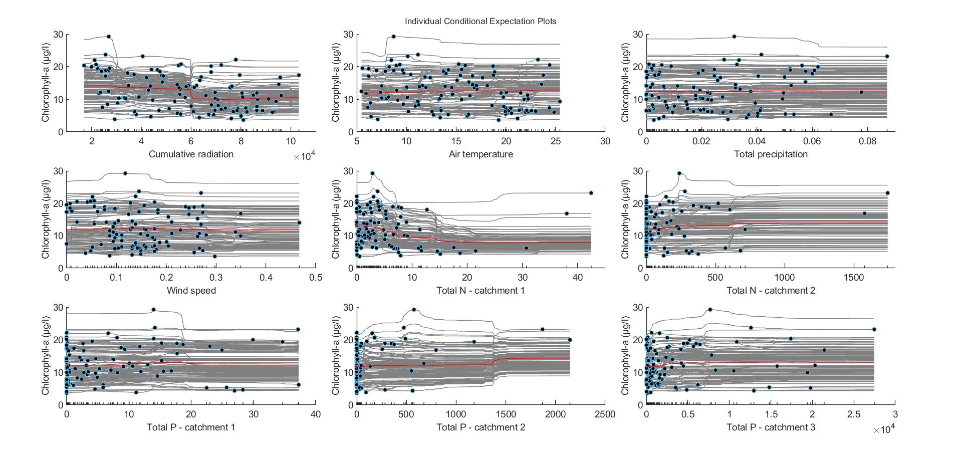
Figure. ICE plots for (a) cumulative radiation, (b) air temperature, (c) total precipitation, (d) wind speed, (e-f) total nitrogen mass fluxes, and (g-i) total phosphorus mass fluxes. Red lines depict the partial dependence of each variable with chlorophyll-a.
AOI4
The RF model provided an adequate representation of the observed chlorophyll-a concentrations. However, it slightly underpredicted the 2019 event and overpredicted concentrations from spring 2017 to summer 2017.
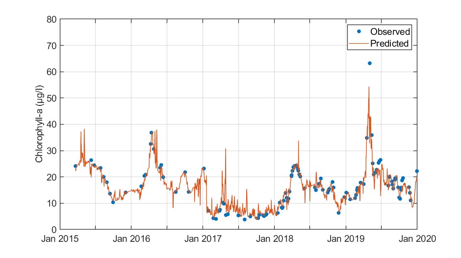
Figure. Observed versus cross-validation predictions of chlorophyll-a.
From the sequential feature selection strategy employed, only total precipitation was removed from the feature list.
The calculated permutation VIMs showed that nutrient influxes (mostly total nitrogen) and air temperature are vital for the trained RF model.
Shapley values indicated towards the same features as essential for AOI4. Total nitrogen and phosphorus influxes from the upstream catchments are primarily driving phytoplankton dynamics in AOI4. However, ICE plots and PDPs could not disentangle how these features impact chlorophyll-a formation. A minor linkage between high total P fluxes and increased chlorophyll-a concentrations exists, however, generalizable patterns could not be inferred by this approach.
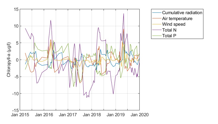
Figure. Shapley values for the predicted chlorophyll-a values.
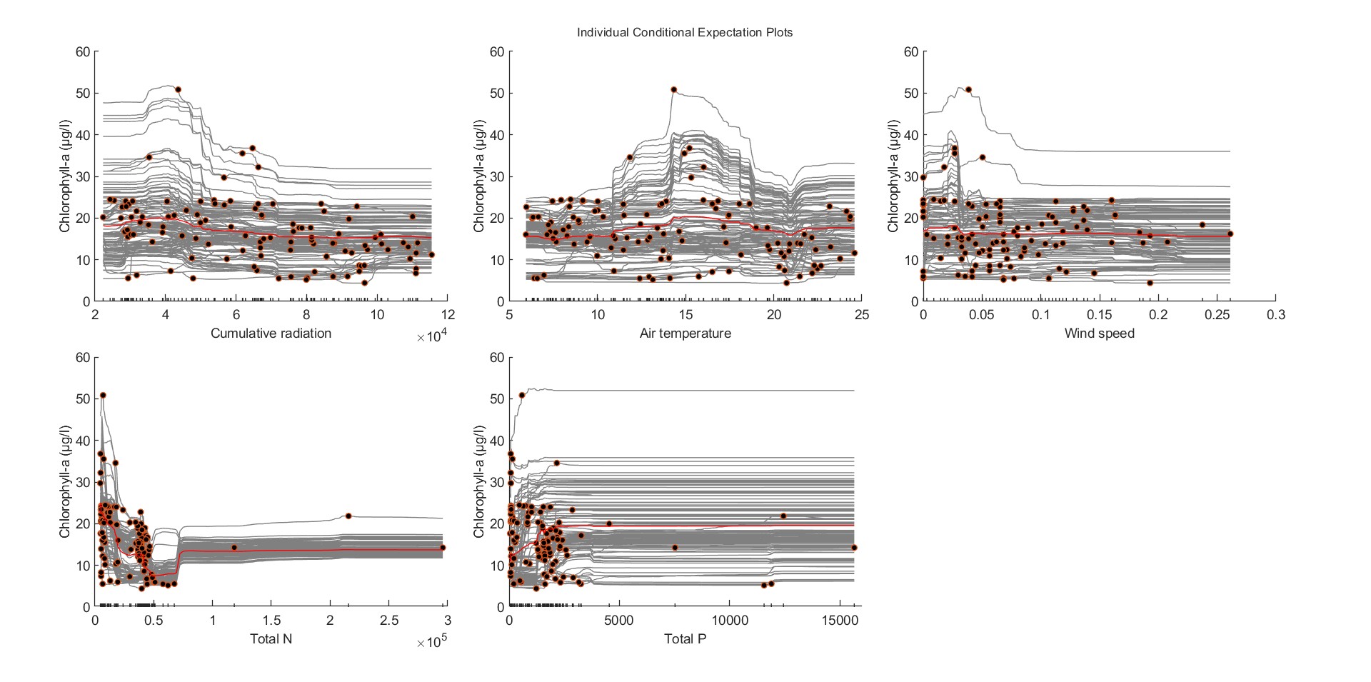
Figure. ICE plots for (a) cumulative radiation, (b) air temperature, (c) wind speed, (d) total nitrogen fluxes, and (e) total phosphorus mass fluxes. Red lines depict the partial dependence of each variable with chlorophyll-a.
This experiment investigated (a) the suitability of medium-resolution, multi-spectral satellite-derived water quality for the development of theory-guided data-driven models of phytoplankton dynamics, (b) how machine learning solutions can valorize satellite-derived data in search for patterns of phytoplankton dynamics in inland waters.
A theory-guided model architecture was adopted using hydrometeorological variables as predictors and chlorophyll-a as the proxy of phytoplankton dynamics. A random forest (RF) model helped to map hydrometeorological variables to chlorophyll-a.
The outputs from three diverse water bodies offered evidence that sufficient multi-spectral satellite data can support the development of data-driven models with reasonable accuracy. For cases with adequate observations, RF models demonstrated reasonable cross-validation errors, and, thus, can be trusted. On the contrary, with limited data available (e.g., due to aerosol, shadow, or cloud contaminations, etc.), predictive performance deteriorated to marginally acceptable levels.
Concerning predictive capabilities, the models capture the temporal dynamics but also tend to underpredict high chlorophyll-a values. To ensure the generalizability of the models, the models were trained to provide smoother approximations of the temporal variability of chlorophyll-a. As a result, the few abnormal chlorophyll-a values were treated as noise, and, thus, the magnitude of peak chlorophyll-a concentrations was not captured.
From the cases tested herein, 100 data records are a rule-of-thumb for the number of data records needed for the development of acceptable models. For less data, data imputation techniques or fusion with alternate data sources (satellite-derived or in situ) should be utilized to populate the available observational data.
A major concern of the experiment is inference and to which degree interpret the relationship between the response variables and the predictor variables.
Concerning the methodological approaches employed for the interpretation of predictions, permutation VIMs offered a useful window into the models’ internals. VIMs were further confirmed by the estimation of Shapley values, which were valuable in understanding the local behavior of the models. Nonetheless, to offer an improved understanding of how hydrometeorological variables may influence phytoplankton dynamics, visualization tools, such as ICE plots and PDPs, are necessary.
Using the abovementioned tools, RFs indicated specific relationships between variables that could explain the temporal variation of chlorophyll-a values in a few areas of the examined water bodies. Yet, for most cases, the models are hard to interpret. Hydrometeorological variables impacted chlorophyll-a predictions in an obscure way, which in many cases contradicted cause-effect relationships that have been well documented.
Conclusively, when sufficient in numbers, medium-resolution, multi-spectral satellite data may be used to develop credible models of phytoplankton dynamics. Using both local and global interpretability tools, these models can provide evidence that explain how hydrometeorological variables lead to phytoplankton outbreaks. However, this is not always feasible due to the highly non-linear nature of the phenomena under examination. When data is insufficient, models may be too simplistic and fail to capture important temporal patterns. In this case, it is difficult to interpret model-based predictions and, thereby, infer meaningful relationships between input and output parameters. In any case, data fusion seems to be a promising path towards the extraction meaningful conclusions on what drives phytoplankton dynamics in inland waters.
Leave a Reply
You must be logged in to post a comment.