
Develop and benchmark data-driven algorithms to forecast the short-term dynamics of phytoplankton in surface water reservoirs
Experiment name:
Develop and benchmark data-driven algorithms to forecast the short-term dynamics of phytoplankton in surface water reservoirs
Scientific question:
How much more accurate can data-driven algorithms be in predicting chlorophyll-a compared to naïve predicting alternatives? What are the limits of predictability in terms of forecasting horizons?
Experiment idea:
This experiment functions as a proof-of-concept for ensemble learning methods in water quality forecasting. The experiment assesses the prediction improvements of an RF algorithm compared to a naïve predicting alternative.


![]()
Ilias PECHLIVANIDIS
[email protected]

Andrea VIRDIS
[email protected]

Blake SCHAEFFER
[email protected]
Background information
Data-driven models are simple in nature, as they do not rely on the a priori knowledge of the processes that drive phytoplankton growth in lake and reservoir ecosystems. Yet, they rely heavily on data availability. When sufficient data are available, data-driven models have been proven as potent tools for short-term (day to weeks) forecasting (Vinçon-Leite and Casenave, 2019; Cruz et al., 2021). Unfortunately, in many cases this lack of sufficient data becomes a major obstacle.
This obstacle motivated the present experiment which leverages existing hydrometeorological data and satellite-derived water quality observations to develop and test alternate data-driven approaches for the short-term forecasting of eutrophication dynamics in lakes and reservoirs. The aim of the present effort goes beyond the development of a data-driven model. In particular, the aim of this experiment aims to test the suitability of data sets that are readily available at a global scale even in data-scarce water bodies: (a) hydrometeorological data that are available from the corresponding global hydrometeorological models, and (b) satellite-derived water quality. In addition, this experiment aspires to evaluate the limits of forecasting capacities using such data sources and models compared to a naïve forecasting alternative.
To these ends, the experiment will first fine-tune the hyperparameters of an ensemble learning approach. It will optimize (a) the minimum leaf size, the number of splits, the number of trees, the number of variables to sample of the ensemble learning model (a Random Forest model in particular) and (b) the formulation of the kernel function, the basis function, the noise variance for the GPR algorithm. Hyperparameter fine-tuning will be performed using a Bayesian optimization method to minimize cross-validation errors of satellite-derived chlorophyll-a predictions in (a) Mulargia reservoir, (b) William H Harsha Lake, and (c) Lake Hume. Model training will be performed using a 5-year-long period (2015-2019). The data-driven algorithms will be trained on (a) simulated hydrometeorological data and (b) earth-observation-derived water quality to predict earth-observation-derived chlorophyll-a concentrations.
Then, the developed models will be evaluated in a re-forecast experiment for the years 2015-2018 using expired short-term forecasts of hydrometeorological variables.
The evaluation of forecasts has several purposes. Evaluation may serve to assign a level of trust in the forecast, to diagnose problems in forecasting models, or to provide an objective function for calibration of the models. In our case, forecast evaluations target to indicate when and why the model succeeds and fails to forecast adequately, and, thereby, assign a level of trust to the forecasts.
It is possible to distinguish three different dimensions of forecast “goodness”: (a) consistency, (b) quality, and (c) value. Consistency is a desirable property, which should be interpreted as the match between the internal beliefs and the external forecast (Weijs et al., 2010). Quality is a dimension that is mostly essential from a scientific perspective, as it concerns evaluating predictions by comparing forecasts with observations. Lastly, value is related to a decision problem attached to the forecast. Value is more closely related to engineering than to science. Therefore, it relies not only on the forecasts and the observations, but also on who is using the forecasts.
Herein we aim to evaluate the quality of ML-based forecasts (as defined above, i.e., identifying their mismatch with observations) paying, however, attention to their adding value for decision-making. The adding value of a forecast can be assessed by how close it was to the observations compared to how close another simple ‘best guess’ alternative (benchmark) was (Pappenberger et al., 2015).
Leader
EMVIS
Short Description
This task collects the available hydrometeorological (predictors) and phytoplankton-related data (target values) for the training of the ensemble learning algorithm at each case study.
Outcome
Hydrological data comprise nutrient fluxes from the upstream catchments. Hydrological data for the three case studies are available through the following link: https://www.primewater.eu/datasets/?_data_type=simulated-hydrology
Meteorological data comprise air temperature at 2 m above surface, solar radiation, total precipitation, and wind speed at 10 meters above surface. Near surface meteorological variables are derived from a bias-corrected reanalysis data set, which can be accessed through the Copernicus Climate Data Store at: https://cds.climate.copernicus.eu/cdsapp#!/dataset/derived-near-surface-meteorological-variables
Satellite-derived concentrations of chlorophyll-a can be accessed through: (a) https://zenodo.org/record/4582339 for Mulargia, (b) https://zenodo.org/record/4581108 for William H Harsha Lake, and (c) https://zenodo.org/record/4581196 for Lake Hume. All data cover a five-year-long period, i.e., 2015-2019, and refer to Landsat-8 and Sentinel-2 retrievals.
Leader
EMVIS
Short Description
In this task, the gridded data for (a) meteorological variables and (b) remotely sensed chlorophyll-a concentrations are formulated as time-series data corresponding to specific areas of interest (AOIs) within the water bodies.
Outcome
Remotely sensed chlorophyll-a concentrations were re-formatted as time series data by averaging chlorophyll-a concentrations within a radius of 200 m around specific areas of interest (AOIs).
For Mulargia reservoir, the AOI is located at (39.6072,9.2547) and corresponds to the water abstraction area of the reservoir.
For William H Harsha Lake two AOIs were specified. They were located at: (39.0367, -84.1381), and (39.020, -84.1311). The two AOIs specified herein represent the two diverse parts of the lake in the east and in the west.
Likewise, four AOIs were selected for Lake Hume. These are located (a) at Heywoods (-36.0711,147.0644), (b) close to the dam wall (-36.1076, 147.034), (c) at the northern part of Hume (-36.0346, 147.1100), and (d) near the Mitta-Mitta arm (-36.1841, 147.0666).
Near surface meteorological variables were estimated at the center of each AOI using the gridded data collected at Task 1 and a nearest neighbor approach through the interp2 command of Matlab®.
Matlab-based scripts for the formatting of input data as time series are available here: https://github.com/EMVIS/ML-Forecasting
The output data formatted in time series are available here: https://zenodo.org/record/7780519
Leader
EMVIS
Short Description
First, this task handles missingness and noise in the target values (i.e., chlorophyll-a). Then, it prepares the training and validation data sets applying a lag and a sliding window strategy for the predictors and the target values. Finally, it normalizes the predictors using z-score.
Outcome
Due to their sparser temporal resolution and the quality-related challenges (e.g., aerosol or cloud contamination) they are facing, satellite-derived time-series contained missing and noisy data. We adopted a two-step approach to handle missingness and noise in those time series. First, we applied linear interpolation scheme; gaps larger than five days were not interpolated and left as missing values, as described in Metz et al. (2017). Then, we applied the Savitzky-Golay filter to smooth noisy inputs.
An integral step of the prediction strategy involved the application of a lag and a sliding window method. The width of the moving window is estimated based on a grid-based search method, where different moving windows are concerned, and cross-validation errors are estimated.
To provide an example of how data are formulated in the prediction strategy, for the day-ahead prediction with a ten-day sliding window, (a) a one-day lag was applied to the target values (the time series of chlorophyll-a concentrations), and (b) the predictor matrix contained statistical indices of the hydrometeorological inputs of the last ten days (i.e., the width of the moving window). These statistical indices were: (a) the cumulative mass fluxes of total nitrogen and total phosphorus entering the reservoir from the upstream catchment areas, (b) the percentage (%) of time during which wind speed exceeds 3.0 m/s – Binding et al. 2018 and Zhang et al. 2021 indicate that a wind-speed threshold of 3.0 m/s is relevant for algae dynamics in lakes and reservoirs, (c) mean air temperature, (d) total solar radiation, and (e) total daily precipitation.
To account for the different scales between predictors (e.g., total precipitation values and total inflow from upstream catchment areas), the predictor set was normalized using Z-score. Z-scores measure the distance of a data point from the mean in terms of the standard deviation. The standardized dataset has zero mean and standard deviation equal to one but retains the shape properties of the original data set (same skewness and kurtosis).
Following normalization, data were split into five partitions to allow for a 5-fold validation during training and safeguard against overfitting. These splits were realized with the cvpartition MATLAB function to obtain a quasi-random draw.
Leader
EMVIS
Short Description
This task searches for a subset of the features in the full model with comparative predictive power through a wrapper method.
Outcome
A Matlab-based script was created to employ a wrapper method for sequential feature selection. Backward direction was used for the sequential search of features assessing the relative change in the cross-validation errors. A feature was removed from the predictor list when its removal induced a change in the cross-validation errors lower than 1% (relative tolerance).
Then, for each case study and each AOI, a subset of the hydrometeorological variables is selected for the development of the corresponding models.
Leader
EMVIS
Short Description
This task optimizes the parameters of the RF and GPR algorithms for each case study and AOI.
Outcome
A Matlab-based script was created to find the hyperparameters of the ML algorithms that minimize the cross-validation errors of chlorophyll-a predictions.
For RFs, development was performed using surrogate splits and an interaction-curvature test for predictor selection, through the Treebagger function of Matlab. Hyperparameter optimization was performed through a Bayesian optimization algorithm (bayesopt function of Matlab). Four parameters were considered adjustable: the minimum leaf size (minLS), the number of variables to sample (nVars), the number of splits (nSplit), and the number of regression trees (nTree).
When growing decision trees to create their ensemble, optimization targets for their simplicity and predictive power. Deep trees with many leaves are usually highly accurate on the training data. However, these trees are not guaranteed to show comparable accuracy for out-of-sample predictions. A leafy tree tends to overtrain (or overfit), and its out-of-sample accuracy is often far less than its training accuracy. In contrast, a shallow tree does not attain high training accuracy. But a shallow tree can be more robust — its training accuracy could be close to that of a representative test set. Also, a shallow tree is easy to interpret. In this regard, the adjustable parameters were constrained to provide shallow trees.
Leader
EMVIS
Short Description
This task runs the RF algorithms in a forecasting rationale and evaluates chlorophyll-a concentrations using expired forecasts for the hydrometeorological predictors for the historical period of 2015-2018.
Outcome
A Matlab-based script utilizes expired shor-term hydrometeorological forecasts (data are available as time-series in https://zenodo.org/record/7890931) from the period 2015-2018 and forecasts chl-a concentrations up to 10 days ahead in the future.
Leader
EMVIS
Short Description
This task calculates the Mean Absolute Scaled Errors for the data-driven algorithms and their naïve prediction alternative.
Outcome
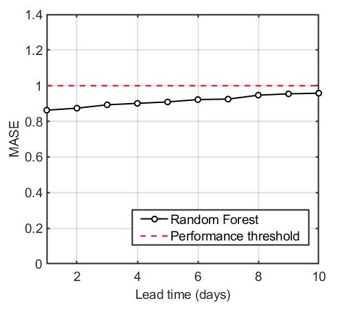
Mulargia reservoir
The RF outperformed its naïve alternative for lead times up to ten days. MASE values ranged from 0.86 to 0.96. Forecasting performance drops slightly with lead time due to forecasting uncertainty introduced by the expired forecasts of the predictors. For lead times greater than 8 days, the RF model produces forecasts that are comparable to the last-known observation alternative.
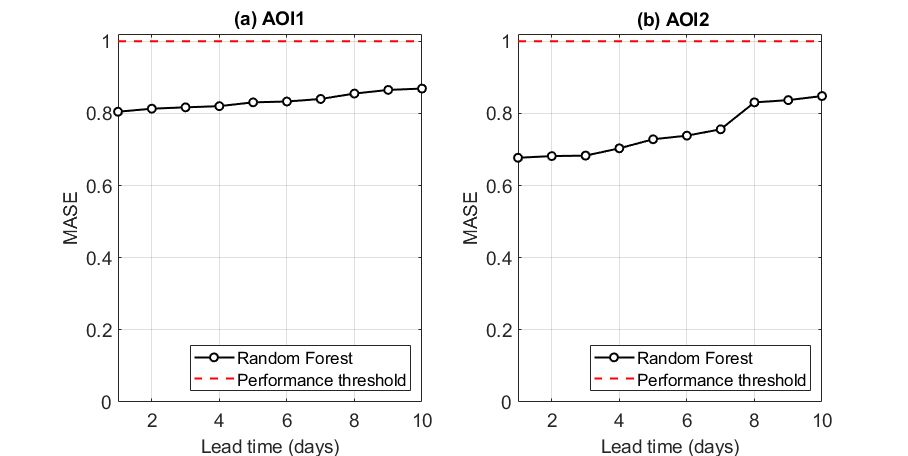
Lake Harsha
In both AOIs, ML algorithms performed adequately in a forecasting mode, outperforming their naïve alternatives.
For AOI1, the RF was better than its naïve alternative for lead times up to ten days, as MASE values ranged from 0.80 to 0.85. The forecasting performance remained relatively steady for all lead times.
For AOI2, the RF was significantly more accurate compared to its naïve alternative for lead times up to three days. It exhibited nearly two-fold lower errors compared to the last-known observation method. For lead times exceeding three days the forecasting skill drops slightly but remains always below 1.0.
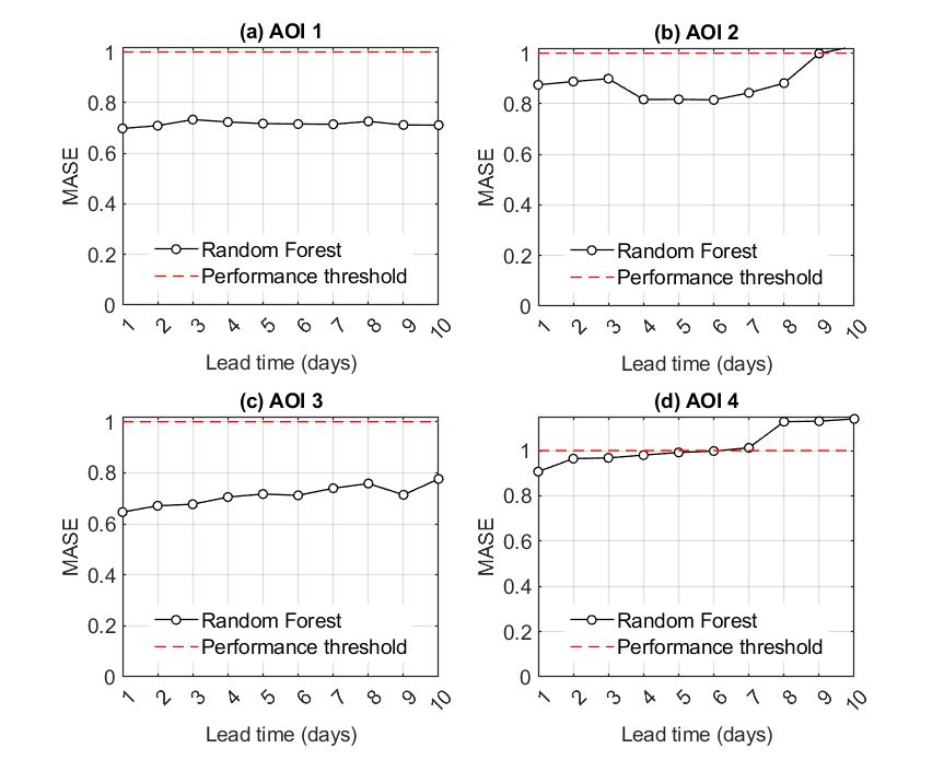
Lake Hume
When compared to the naïve alternative, for AOI1 and AOI2, the RF-based forecasts were more accurate for lead times up to ten days. For AOI3, the RF model outcompeted the naïve alternative for forecasts up to eight days ahead. Lastly, for AOI4 the RF model provided meaningful forecasts only for a lead time of one day. After this forecasting horizon, the performance of the RF model drops and is comparable to the persistency method, which functions as the naïve alternative. After six days ahead, sticking to the last known observation is preferable.
Models that are intended to support decision-making processes need to be evaluated in terms of the degree of similarity between them and verification data.
Another imperative component is the evaluation of the models in forecast mode. In this case, it is relevant to evaluate whether the forecasts add value compared to other data sources that are available to end users. The adding value of a forecast can be assessed through a benchmarking analysis.
This experiment aims to evaluate the value of alternate data-driven models compared to a naïve forecasting alternative, i.e., the persistency of the last available observation. Benchmarking was performed at all AOIs in three case studies for deterministic point forecasts using Random Forests.
When compared to a naïve alternative, the RF-based forecasts were more accurate for lead times up to six days ahead for all cases. For greater lead times, there were cases in which the persistency of the last available observations would be preferable.
It should be noted, however, that this approach did not evaluate the relevance of bias adjustments in the model’s inputs. This highlights that even without any type of adjustments, the RF model remained adequately robust to provide trustworthy forecasts
Leave a Reply
You must be logged in to post a comment.