
Assimilation of Earth Observation products in water quality modelling
Experiment name:
Assimilation of Earth Observation products in water quality modelling
Scientific question:
Can we combine EOs and enKF/4dVAR data assimilation techniques to improve the predictive skill of hydro-ecological modelling in reservoirs?
Experiment idea:
The first round of experiments is centered around optimizing the EnKF data assimilation approach using in-situ data. The EnKF algorithm incorporates observations from in-situ sensors placed within the lake to assimilate data into the model. By carefully analyzing and refining the algorithm, the objective is to enhance the accuracy of chlorophyll-a predictions by effectively integrating the in-situ measurements.
In the second round of trials we focus on integrating EO data into the EnKF data assimilation framework. EO data provides a wider spatial coverage and complements the in-situ measurements. By assimilating EO data into the EnKF algorithm, the objective is to improve the model’s predictive capabilities utilizing EO measured chlorophyll-a, assessing how modifying the parameterization of enKF is affecting the conveyance of the correction both on the spatial and temporal scale.
Lastly, the experiments explore the application of the 4DVar data assimilation method using in-situ data. The 4DVar algorithm utilizes a variational approach to assimilate observational data over a specified assimilation window, accounting for both the model dynamics and measurement uncertainties. The objective is to enhance the accuracy and consistency of chlorophyll-a predictions throughout the assimilation window, capturing the temporal evolution of chlorophyll-a concentrations more effectively.

Marcos Julien ALEXOPOULOS
[email protected]
Evangelos ROMAS
[email protected]
Apostolos TZIMAS
[email protected]

![]()
Ilias PECHLIVANIDIS
[email protected]

Andrea VIRDIS
[email protected]

Blake SCHAEFFER
[email protected]
Background information
Experiment B2 investigates how in-situ and satellite observations can improve the skill of short-term forecasting of water quality characteristics in surface water reservoirs through data assimilation (DA) techniques in three-dimensional, process-based reservoir models.
All process-based models are based on simplifications of the reality and therefore introduce errors between the predicted and observed quantities. Data assimilation is often thought of as a way of keeping a model ‘on the tracks’ by constantly providing the optimum combination of the available information to produce the most realistic state of the modelled system just before a new forecast model is going to be launched. This state is expected to yield the best possible forecast.
The 4DVar method is a variational data assimilation method that considers observations over a specified assimilation window. It aims to find the best agreement between the model trajectory and both the background and observational data within this window. By optimizing the initial conditions of the model, 4DVar adjusts the trajectory in space and time, leading to a closer alignment with the observations. However, the implementation of 4DVar requires coding and maintaining tangent linear and adjoint models, which can be computationally challenging, especially for complex hydrodynamic and water quality models.
The EnKF method belongs to the family of sequential data assimilation methods. It propagates the error covariance of a non-linear model by using an ensemble of model trajectories. Each ensemble member represents a probability density function and is treated as a unique estimate for the next state. The EnKF method allows for the assimilation of observations as soon as they become available, updating the model state in both observed and unobserved cells based on the covariance information.
The experiment is conducted for a 1-year-long period (2018) in Lake Harsha using the Delft3D suite for the three-dimensional hydrodynamic and water quality simulations of the two cases. The models are setup and calibrated using all available datasets including EO-based water quality products from Landsat 8 and Sentinel 2 (e.g. water temperature, chlorophyll-a concentrations, turbidity) as well as measurements from in-situ stations and monitoring campaigns.
The assimilation algorithms are developed within a computational environment that allows their dynamic coupling with the Delft3D suite for the implementation of the experiments. This enables the efficient configuration of the DA methods for the selected reservoir and the investigation of several critical parameters (e.g., ensemble size and noise levels, estimation of background covariance error, length of assimilation period) that affect their performance. A series of DA-enabled simulations is performed to improve model parameter chlorophyll-a. A series of model evaluation metrics are used to quantify the performance gain of the assimilated vs the non-assimilated versions of the water quality model.
Leader
EMVIS
Short Description
The chlorophyll-a measurement files were edited and manipulated for the EnKF in situ trials. The files used for validation were separated from the files used for correction conveyance to avoid bias in performance evaluation. Additionally, specific subsets of files were curated based on the trial objectives. Similar manipulations were performed for trials involving the validation of the vertical column, repeated single-station runs, and multiple station trials.
Outcome
The produced datasets are open source and can be accessed ![]()
Leader
EMVIS
Short Description
In the EO trials, the chlorophyll-a estimates from satellite products needed to be resampled to match the Delft3D model grid. The main chlorophyll-a value for each in-situ station was determined using the corresponding coordinates. To incorporate this value within each cell of the representative station, a resampling procedure was applied. This involved averaging the neighboring pixels of each image over a radius of 150 m, with the primary chlorophyll-a value at the center. This procedure ensured consistency with each satellite product and provided a single value within the 100x100m cells in the Delft3D model. The resampling process varied slightly between Sentinel-2 and Landsat-8 images due to their different resolutions. For the trials involving varying radii and lake partitioning, an inverted procedure was implemented. Circular radii were selected and applied within the Delft3D model at the location of each in-situ measurement station. These radii concealed the state of chlorophyll-a, with each measurement station corresponding to the midpoint of the radius. Using the covariance matrix in the EnKF scheme, the centers of these radii received a correction from the non-masked pixels of satellite images containing chlorophyll-a estimates.
Outcome
The produced datasets are open source and can be accessed ![]()
Leader
EMVIS
Short Description
Assess the effectiveness of EnKF in assimilating chlorophyll-a measurements from in-situ stations and evaluate the optimal number of stations for correction conveyance.
Outcome
1. The EnKF algorithm successfully corrects chlorophyll-a simulation using in-situ measurements, with a single station capable of efficiently correcting most of the domain.
2. Correction is most effective when conveyed at respective depths.
3. The correction performance is influenced by the similarity of characteristics and nutrient properties between contributing and receiving stations.
4. Multiple stations do not necessarily lead to significant performance enhancement, and a single station achieves better results.
Leader
EMVIS
Short Description
Investigate the application of EnKF using EO data for chlorophyll-a assimilation and explore the influence of radius, covariance matrix augmentation, and lake partitioning.
Outcome
1. Assimilation of EO data through EnKF shows a slight decrease in simulation performance compared to in-situ observations.
2. Varying radii during assimilation reveals that a 600m radius leads to slightly better performance.
3. Augmenting the covariance matrix by including additional layers provides a slight improvement in the model’s performance.
4. Partitioning the lake modeling into western and eastern sections highlights the better correction conveyance in the western subgroup.
Leader
EMVIS
Short Description
Evaluate the application of 4DVar for chlorophyll-a assimilation and optimize its configuration, including perturbation intervals, nutrient sensitivity, and horizontal discretization.
Outcome
1. Optimal perturbation intervals of 15 and 8 days are identified, indicating the timeframe for achieving convergence with observed values.
2. A moderate range of perturbation (0.2 μg) for nutrient variables yields the best simulation results.
3. Horizontal discretization reveals that two layers offer better simulation accuracy and observation fitting.
4. Comparison with EnKF indicates that EnKF performs better in correcting deeper depths, while 4DVar excels in estimating a specific point of interest across the entire depth.
Leader
EMVIS
Short Description
Assess the effectiveness of EnKF in assimilating chlorophyll-a measurements from in-situ stations and evaluate the optimal number of stations for correction conveyance.
Outcome
1. The EnKF algorithm successfully corrects chlorophyll-a simulation using in-situ measurements, with a single station capable of efficiently correcting most of the domain. A level plot, containing the RMSE difference score, is illustrated in Figure 1. This score is deduced from the performance pre- and post-assimilation for each run identified by its station name. The level plot depicts the performance of the EnKF scheme in the rest of the remaining cells, with NA values indicating the absence of station performance whenever the same station is used to provide information during model propagation. Each column reflects the station that contributes information during model propagation, and rows signify validation stations. Positive RMSE difference scores imply a performance increase in the station, while negative scores indicate performance aggravation.
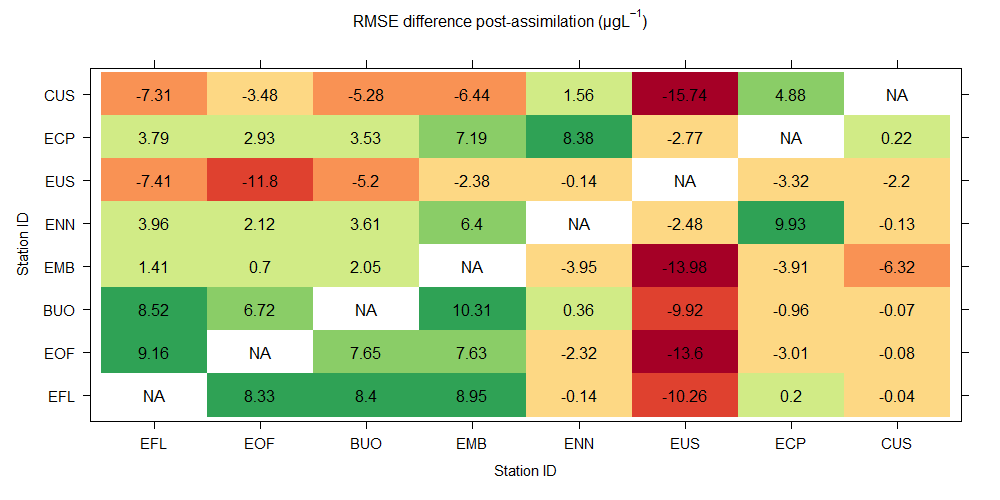
Figure 1. Levelplot displaying the RMSE skill per each contributing buoy station
The EUS station measurements significantly deteriorate the performance of most of the remaining stations, with the majority of stations that provide added value located in the western part of the modelling domain, closer to the outlet. Specifically, the EFL, EOF, BUO, and EMB stations enhance chlorophyll-a estimations to all stations, except for the EUS and CUS stations, which are situated in the inlet reaches of the lake. In contrast, the ENN and ECP stations located in the eastern domain improve performance in only three of the remaining seven stations. No significant trends are observable, but stations located in the eastern part mostly optimize stations enclosed in the same area. 50% of employed stations effectively contribute to 75% of validation cells, and a single observational point is sufficient to correct most of the modelling domain. The inability of certain stations to contribute and receive the correction is likely due to the different properties of the eastern and western parts of the lake model, which warrants further research.
2. Correction is most effective when conveyed at respective depths. Figure 2 displays the pre- and post-assimilation chlorophyll-a time series for the EOF station. As the model follows the discretization scheme previously described, each layer is not guided by neighboring layers. However, this leads to chlorophyll-a concentration paths that deviate from their original paths without providing accurate estimates that match the observed values. This effect is most pronounced in the deepest layer (Layer 03). Extracting observations from the bottom layer results in model paths that match measurements exclusively for Layer 03, but in the present configuration, concentrations closely match observations, except for the significant underestimation on the 24th of April. For Layer 02, modeled concentrations miss the same observation, in addition to the observation measured on the 20th of June. The correction leads the model estimates closer to the observations for the remaining observations. However, the path in Layer 03 still slightly deviates from the pre-assimilation path, indicating that the correction is not permanent and concentrations eventually revert to their original path. This effect is more evident in the July record, where the algae bloom is at its peak.
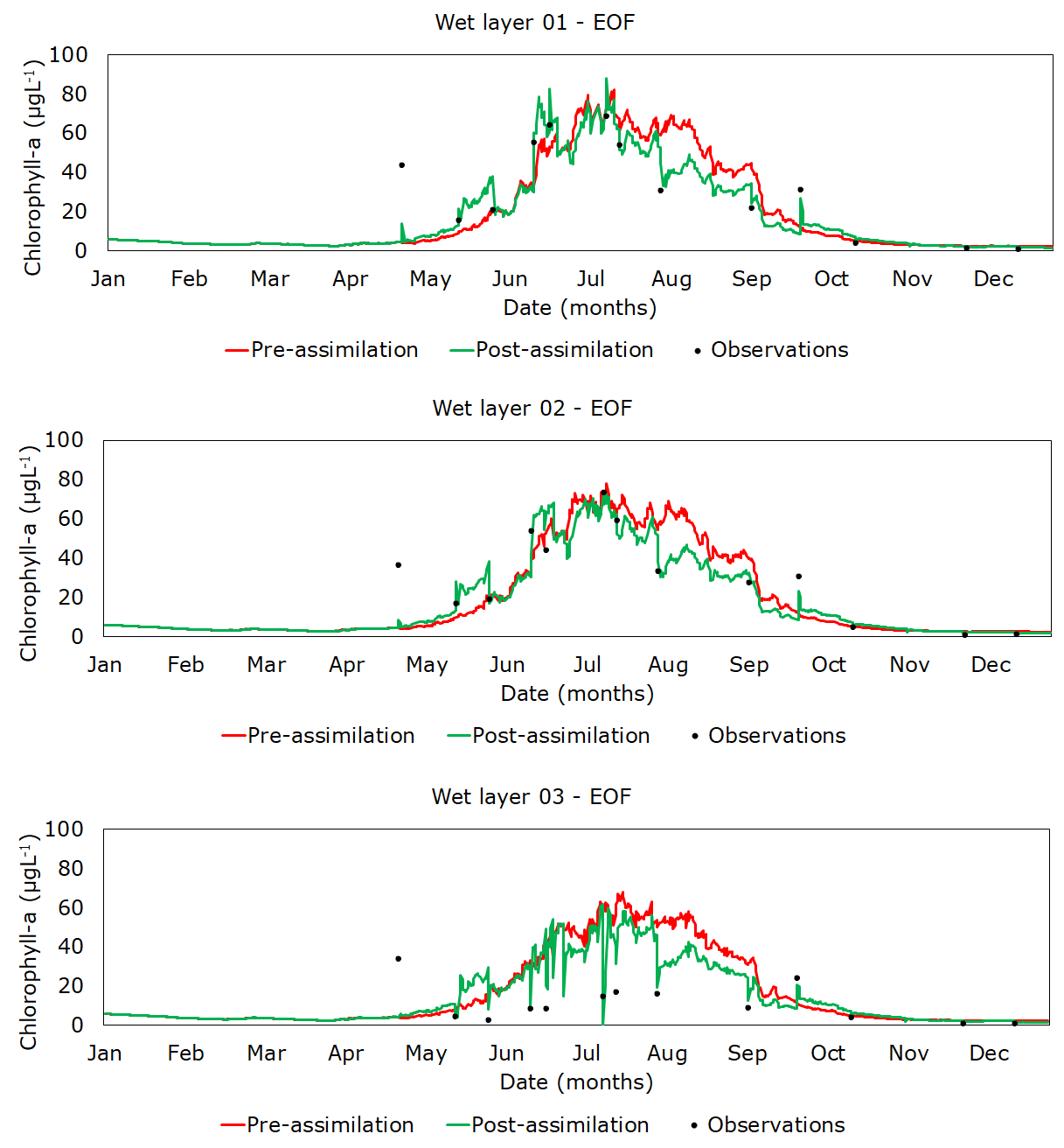
Figure 2. Pre- and post-assimilation chlorophyll-a solution against observations – EOF station – Layer 01, 02 and 03
3. Multiple stations do not necessarily lead to significant performance enhancement, and a single station achieves better results. Figure 3 displays chlorophyll-a time series in the EOF station post-assimilation, derived from one and three contributing stations, for Layer 01, 02 and 03.
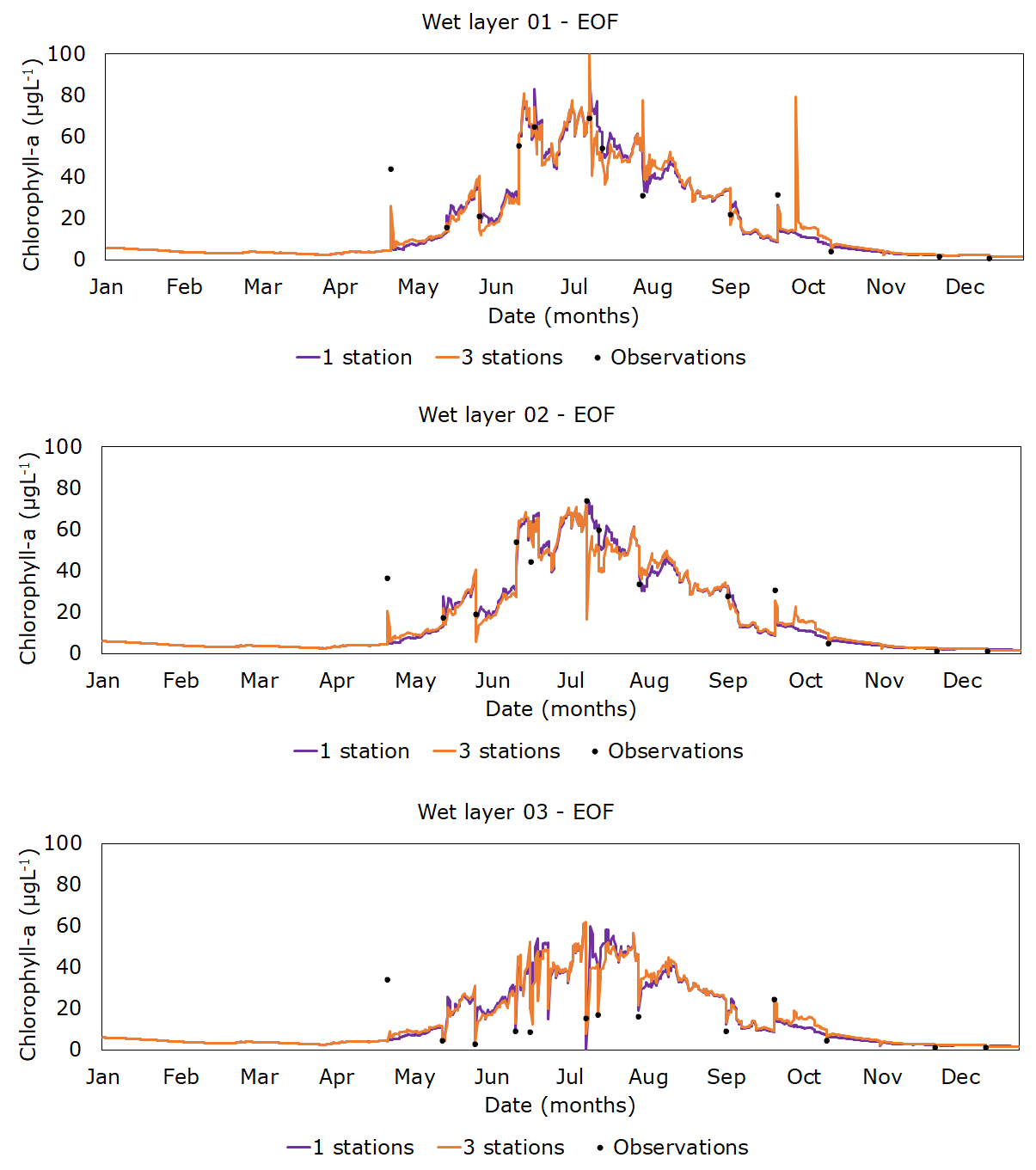
Figure 3. 1- and 3-station mean chlorophyll-a solutions against observations – EOF station, Layers 01, 02, 03
The presented analysis showcases a notable fluctuation in the orange line corresponding to the time series produced by the assimilation of measurements from three observation sites, across all three layers, regardless of their depth. This variation is a consequence of the weighted covariance between the EOF and the BUO-EMB-EFL stations. A clear manifestation of this phenomenon is illustrated in Layer 01, where the concentration values attain a peak of about 80 μg/L on the 2nd of October, despite the absence of a measurement.
Leader
EMVIS
Short Description
Investigate the application of EnKF using EO data for chlorophyll-a assimilation and explore the influence of radius, covariance matrix augmentation, and lake partitioning.
Outcome
1. Assimilation of EO data through EnKF shows a slight decrease in simulation performance compared to in-situ observations. The results of the run reveal that the performance of the model is significantly influenced by the type of measurements used for data assimilation. The total RMSE (Table 1) shows that the model’s overall skill is worsened by approximately 7 μg/L when the EO observations are used instead of in-situ observations. However, it is worth noting that there are variations in model performance across the seven monitoring stations. The EFL and CUS stations show a significant improvement in the model’s ability to replicate EO observations, with a reduction of 4.15 μg/L and 2.94 μg/L, respectively.
Table 1. Pre-assimilation RMSE against in-situ and EO observations
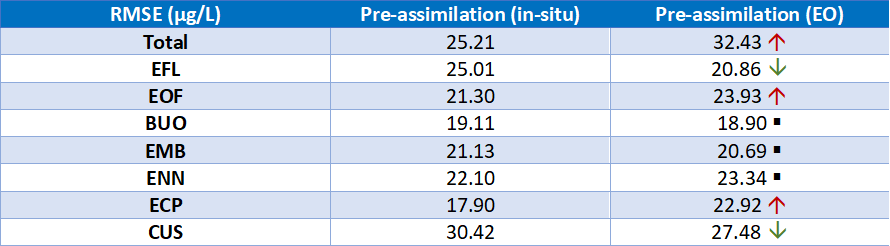
On the other hand, other stations show no significant improvement, and in some cases, such as the EOF station, the RMSE value is slightly higher than the pre-assimilation value, implying that the assimilation of EO observations might have led to a worse model prediction. This suggests that the assimilation of EO observations to improve model performance might not be a straightforward process and depends on various factors such as the location of the monitoring station, characteristics of the observation data, and the model’s parameters. It is worth noting that the assimilation process is dynamic, and future runs could yield different results depending on the input data and other factors that influence the model’s performance.
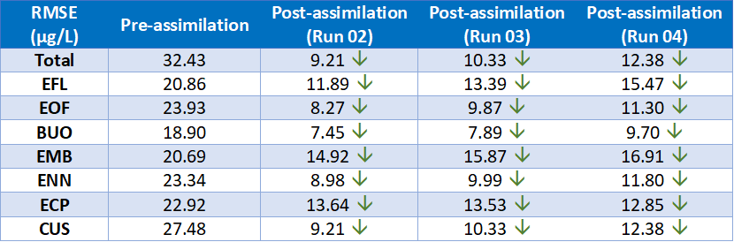
2. A radius of 600m yields slightly better performance during assimilation. Runs 02, 03 and 04 correspond to a radius of 600, 800 and 1000 m, respectively. The results of the RMSE of each run against the pre-assimilation run show that all three runs lead to significant performance enhancements (Table 2). The use of a 600 m radius leads to slightly better performance than the 800m and 1000m radius, but all three are successful.
Table 2. Pre- and post-assimilation RMSE skill for Runs 02, 03 and 04
The plot (Figure 1) displaying the graphs for the BUO station – Layer 01 shows that the post-assimilation path of the mean chlorophyll-a time series is not fluctuating greatly with the addition of the distance within the radius, indicating that the enlargement of the radius during the EnKF application is not significant. It should be noted that the two observations in early December are inconsistent with the general trend of the observations during fall and winter, and may be due to faulty measurements caused by cloud presence during their time of observation. The results show that the chlorophyll-a measurements in the three topmost layers are consistent with each other to a great extent. Nonetheless, it is to be noted that with the increase in radius, a minor deviation from the observations is observed. Specifically, it is observed that the time series for 600 m and 800 m radii are highly consistent with the measured observations, while the time series for 1000 m radius tends to deviate slightly more from the observations. The slight deviation in the time series of the 1000 m radius can be attributed to the integration of a larger set of pixels in the ensemble Kalman filter scheme, which results in increased noise in the assimilated data.
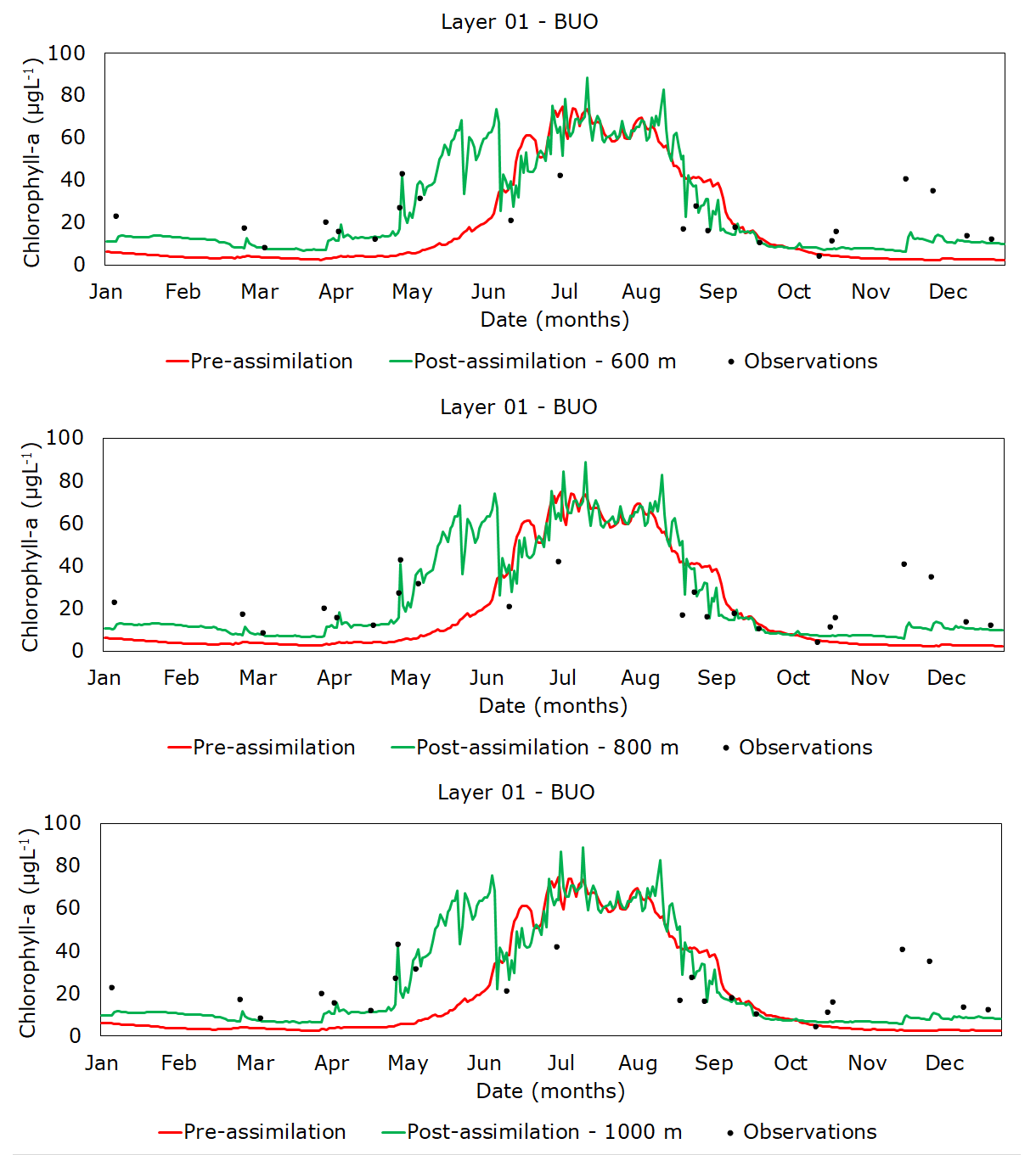
Figure 1. Pre- and post-assimilation time series against observations for Runs 02, 03 and 04
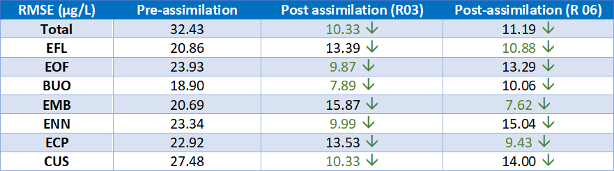
3. Augmenting the covariance matrix with additional layers improves the model’s performance. The results show mixed outcomes (Table 3), where the overall skill is slightly exacerbated. However, when investigating amongst the stations, no visible patterns are present. Runs 03 and 06 correspond to the application of the 800 m radius, with run 06 including layer 03 in the covariance matrix. Although, including the Layer 03 for the formation of the covariance matrix seems to be beneficial when receiving corrections from 800 m radius solely for stations EFL, EMB, and ECP. Nevertheless, no conclusive remarks can be made based on their spatial location within the lake.
Table 3. Pre- and post-assimilation RMSE skill for Runs 03 and 06
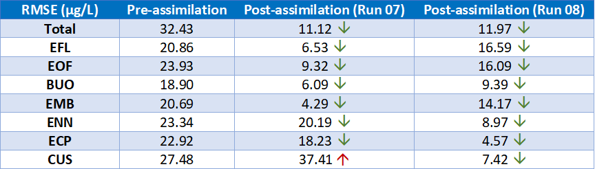
4. Lake partitioning reveals better correction conveyance in the western subgroup. The results of Runs 07 and 08 (western and eastern partitioning) reveal the following observations regarding the EnKF data assimilation process, and the impact of partitioning the Harsha Lake modelling into western and eastern sections. The total RMSE values decrease significantly after correction, as evidenced by the post-assimilation RMSE values for both runs (Figure 5). Notably, the stations located in the western part of the domain show a more significant reduction in RMSE values after correction, when compared to the eastern stations. Specifically, the BUO, EMB, EFL, and EOF stations on the western side of the lake experience an average RMSE reduction of 14 μg/L, while the same stations on the eastern side show a milder reduction of around 7 μg/L.
Table 4. Pre- and post-assimilation RMSE skill for Runs 07 and 08
These findings suggest that each sub-group responds better to the EnKF data assimilation process when receiving corrections from the same partitioned quadrant of the lake. Moreover, the western subgroup is more receptive to corrections overall, which may be attributed to the different dynamics of Lake Harsha. The findings outlined in 1.4.3, has suggested that the eastern part of the lake experiences more riverine dynamics, while water circulation in the western part is milder. The observed differences in RMSE reduction may reflect these different dynamics.
Overall, the findings suggest that partitioning the lake modelling into western and eastern sections may aid in optimizing the EnKF data assimilation process for the present case study, and that prior lake dynamics remain relevant even when using EO data.
Leader
EMVIS
Short Description
Evaluate the application of 4DVar for chlorophyll-a assimilation and optimize its configuration, including perturbation intervals, nutrient sensitivity, and horizontal discretization.
Outcome
1. Optimal perturbation intervals of 15 and 8 days are identified for achieving convergence with observed values. Figure 27 offers a detailed portrayal of the state of chlorophyll-a for the designated time frame spanning from 07/12/18 to 08/03/2018 in Layers 01, 02 and 03. In particular, Figure 27 demonstrates the observations that were recorded at the EOF station for all three layers. Additionally, Figure 27 showcases the time series of chlorophyll-a prior to assimilation, as well as post-assimilation for perturbation windows of fifteen, eight, five and two days. Upon close inspection of each time series, it becomes quite evident that each one commences to deviate from the pre-assimilation time series in accordance with the length of the perturbation window.
Moreover, it is worth noting that the original model state is significantly overestimating the true chlorophyll-a concentration, as evidenced by the respective overestimations of approximately 28, 19 and 28 μg in Layers 01, 02 and 03, respectively. Interestingly, it has been observed that as the initial conditions are shifted further back in time, the concentration of chlorophyll-a gradually decreases and converges closer to the instrument’s observed value. This phenomenon is particularly noteworthy in Layer 02, where the model’s initial skill level is at its best.
It is also pertinent to note that the state of the model is not proportionally brought closer to the observations as the perturbation window is extended. For instance, the time series of the 8- and 15-day intervals appear to behave quite similarly, despite the significant difference in their respective time lengths.
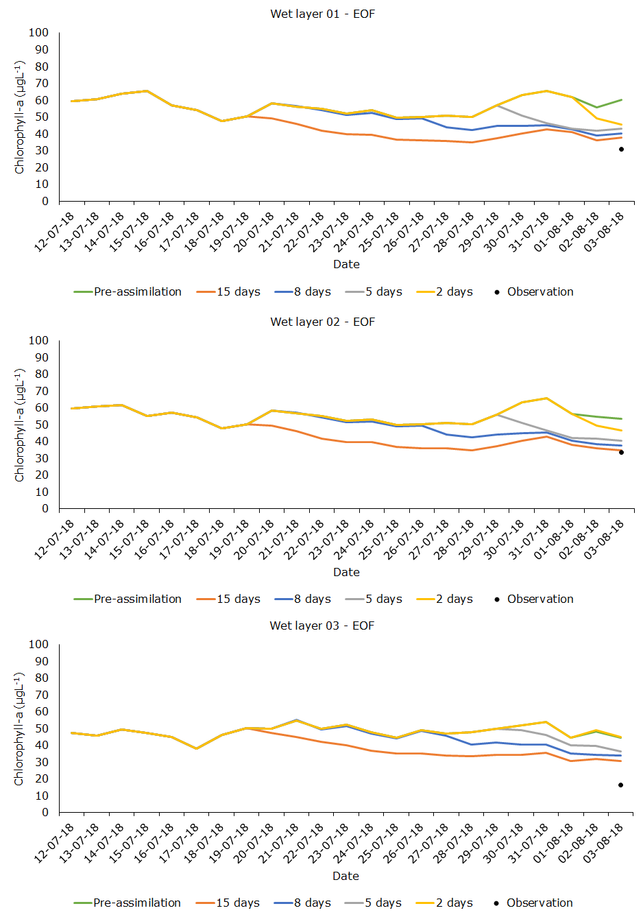
Figure 1. Deviation of runs against pre-assimilation run and observations – EOF station – Layer 01, 02, 03
2. A moderate range of perturbation (0.2 μg) for nutrient variables yields the best simulation results. Figure 2 showcases the time series of chlorophyll-a for each run, including pre-assimilation, alongside the observed values in the EFL station for Layers 01, 02, and 03.
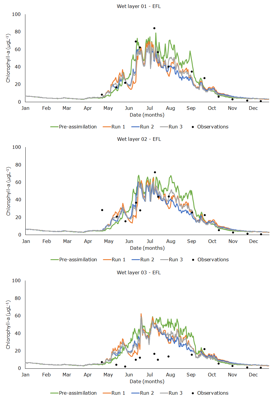
Figure 2. Deviation of runs against pre-assimilation run and observations – EFL station – Layer 01, 02, 03
It appears that the pre-assimilation run is closer in Layer 01 and does not benefit from the 4DVar assimilation scheme when evaluating the model performance for the entire year. While the assimilation scheme improves the performance in Layers 02 and 03, the post-assimilation runs still exhibit certain deficiencies. Specifically, in Layer 01, the model tends to miss some observations while fitting others. For instance, Runs 01, 02, and 03 are shifted downwards by approximately 23 μg/L to fit the observation on 03/08, but this shift leads to an underestimation of the observation on 07/09 by 11 μg/L. Similar inconsistencies are observed in the months of May, June, and July as well as in Layer 02. In Layer 03, while the tabulated values suggest an improvement in the RMSE skill, the model still tends to overestimate by an average of 12 μg/L.
3. Two layers offer better simulation accuracy and observation fitting during horizontal discretization. Table 1 displays the RMSE score for each vertical discretization scheme for the entire domain, and in respect to the Layers. Runs 01 02 and 03 refer to the discretization of 1, 2 and 3 slices, respectively. The data presented in Table 1 provides clear evidence of the superiority of the initial vertical discretization of the modelling domain into two layers.
Table 1. Comparison between pre- and post-assimilation runs with respect to layer
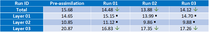
The use of this classification scheme results in a significantly improved overall skill of the model, as compared to other classification schemes. Specifically, any other classification scheme results in a degradation of performance in Layer 01. While the two-slice scheme leads to a slightly higher RMSE score in Layer 03, a single-layer classification is superior by approximately 1 μg. However, in the shallower depths of the lake, the two-slice scheme is deemed superior, as it enables the model to more accurately capture the dynamics of chlorophyll-a concentrations in these areas.
4. 4DVar excels in estimating a specific point of interest. While enKF is able to make use of specific portion of the buoy selection, the 4DVar is able to correct points of interest that do may be characterized by different ecosystem patterns. Figure 3 showcases the temporal variations of chlorophyll-a and nutrient time series, including NH4, NO3, and PO4, generated by both the EnKF (Single station – EMB) and 4DVar algorithm at the EUS station – Layer 01. It is noteworthy that the post-assimilation chlorophyll-a time series obtained from the 4DVar algorithm are capable of capturing the general trends of the observed values, demonstrating the superior skill of this algorithm in representing the chlorophyll-a dynamics at this particular location. Nonetheless, the 4DVar algorithm tends to overestimate the chlorophyll-a measurements during certain periods, such as 30/05 and 28/06, indicating that the model requires further refinement to better fit these observations.
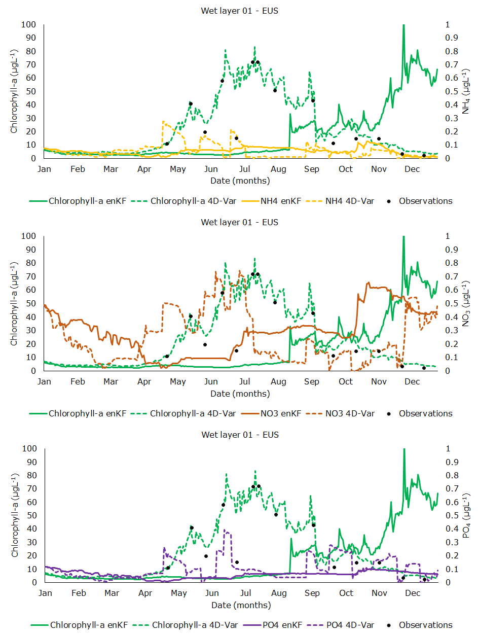
Figure 3. Mean EnKF and 4DVar chlorophyll-a solution, along with nutrients per DA scheme – EUS station – Layer 01
The EO data assimilation using the EnKF scheme demonstrates that validation against EO observations results in a slight decrease in overall skill compared to in-situ observations. Furthermore, experiments on the radius effect, covariance matrix augmentation, and lake partitioning provide insights into optimizing the data assimilation process. The inclusion of Layer 03 in the covariance matrix formation leads to a slight improvement in the model’s performance. Additionally, partitioning the lake into western and eastern sections shows that the western subgroup responds better to corrections.
In the 4DVar scheme, the optimal perturbation intervals for achieving convergence with observed values are identified as 15 and 8 days. Narrow bounds in the search space hinder the optimizer’s ability to find the optimal solution, while excessively large bounds lead to over-perturbations. Horizontal discretization with two layers yields better simulation accuracy and observation fitting. Comparing the 4DVar scheme with the EnKF scheme, we observe that the EnKF is more effective in correcting deeper depths, while the 4DVar algorithm excels in estimating a specific point of interest across the entire depth.
Leave a Reply
You must be logged in to post a comment.